WIP… Exploring Markov Chains

Background

When building a discrete predictive model, it’s natural to assume that adding more features will improve performance. Complex neural networks in particular seem to demand large feature sets and deep historical data to generate accurate predictions. However, high performance doesn’t always require that degree of complexity.

A Stochastic Process describes a system where state changes are driven by probability. This type of process follows an assumption known as the Markov Property - the next state of the system depends only on the current state, not the sequence of prior states that led to the current state. This idea forms a core framework in probabilistic modeling.

A First-Order Markov Chain is a mathematical model that uses this property to predict the next state of a system given only its current state. Despite the simplicity in requiring no memory of past states, this approach can prove powerful across many applications, like natural language processing or predicting how users navigate websites.

The Basics of a Markov Chain

Before we look at a real-world application of a Markov chain model, let’s familiarize ourselves with some basic concepts. For any stochastic process, we must define the State Space S: a complete set of states covering all possible system outcomes. For example, let’s define a system with exactly three states. Then the state space S = {S₁, S₂, S₃}. From any state S_n in S, the system can transition to one of the other two states, or remain in the same state.

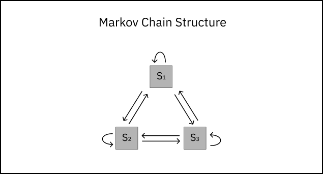
A transition from state i to state j is written as i→j. Consider a random state in our system like S₁. From S₁, there exist three possible transitions:

S₁→S₁ : starting from state S₁, we stay in state S₁.
S₁→S₂ : starting from state S₁, we transition to state S₂.
S₁→S₃ : starting from state S₁, we transition to state S₃.

Each transition i→j has a transition probability - the likelihood of transitioning from state i to state j. The transition probability P_ij can be written as:

P_ij = P(S_i→S_j) = P(S_t+1 = S_j | S_t = S_i) where t indicates a state-step in the system.

In order to estimate the probability of a transition occuring, P̂_ij, we must first observe the system and count the number of transitions from i→j that occur. These observable counts are denoted c_ij.

We’ll also need to count the number of transitions from i→k that have occurred, where k denotes any possible transition state from i. We can denote the total count of transitions from i as c_ik. Now, we’re ready to estimate the transition probability P̂_ij. The maximum likelihood estimator for Markov chain transition probabilities is:

P̂_ij = c_ij / ∑_k c_ik

Once calculating P̂_ij for every possible transition in the system, we can update our original diagram with transition probabilities.

Note: The transition probabilities from any state add up to one, ensuring all possible next states are accounted for.

Application

To recap, Markov chain models are useful when a system’s future state depends primarily on its current state rather than its full history. Compared to more complex models, they require fewer features (and fewer assumptions about their correlations) while maintaining interpretability of state-to-state dynamics.

Let’s dive into a real use case - modeling user navigation on an online retailer website. Here is a visual of the website’s homepage highlighting possible user navigations (states) for the Markov chain.

UI design generated by Claude Sonnet 4.6

I simulated a dataset capturing 10,000 individual user sessions on this website. By defintion, every user journey will start on one of three pages: the homepage (95% of sessions), the search page (3%), or the customer support page (2%). The dataset contains three columns.

session_id is the unique ID for each user session.
t is the click number from the start of a user session.
state is the web page the user navigates to.