
R: Variable Selection in Logistic Regression Modeling
Background
The objective of this project was to determine an optimal logistic regression model for predicting whether a patient had adult-onset diabetes based on certain diagnostic measurements. This dataset was downloaded from Kaggle and originally comes from the National Institute of Diabetes and Digestive and Kidney Diseases. All patients in the data set are females of Pima Indian heritage and at least 21 years old. I was assisted on this project by Dr. Qingning Zhou from the Mathematics and Statistics Department at UNC Charlotte.
Exploratory Data Analysis
We must first import the dataset from Kaggle. Three of the field names from the original data set were rather lengthy, so we can alias them with more appropriate names.
library(readr)
dia <- read_csv("~/Diabetes Research/diabetes.csv")
names(dia)[c(3,4,7)] = c("Bpsi", "Skin", "DPF")
Pregnancies expresses the number of pregnancies per individual. Glucose expresses their glucose level. Bpsi expresses their blood pressure measurement. Skin expresses the thickness of their skin. Insulin expresses the insulin level detected in their blood. BMI expresses body mass index. DPF expresses a numeric value calculated by a diabetes pedigree function that determines the risk of type 2 diabetes based on family history (higher values indicate a higher risk). Age expresses the individual’s age. Outcome is a binary variable expressing the result of having Type 2 diabetes (denoted by 1) or not (denoted by 0).
Next, we can take a look at the distributions of each field in the dataset.
summary(dia)
dia.df = as.data.frame(dia) # changing the list into a data frame
par(mfrow=c(3,3))
for(i in 1:9){
  hist(dia.df[,i], xlab=colnames(dia.df[i]), main=paste("Histogram of", colnames(dia.df[i])), col="lightgreen", breaks=30)
  }
##  Pregnancies        Glucose           Bpsi             Skin          Insulin           BMI             DPF              Age           Outcome
## Min.   : 0.000   Min.   :  0.0   Min.   :  0.00   Min.   : 0.00   Min.   :  0.0   Min.   : 0.00   Min.   :0.0780   Min.   :21.00   Min.   :0.000
## 1st Qu.: 1.000   1st Qu.: 99.0   1st Qu.: 62.00   1st Qu.: 0.00   1st Qu.:  0.0   1st Qu.:27.30   1st Qu.:0.2437   1st Qu.:24.00   1st Qu.:0.000
## Median : 3.000   Median :117.0   Median : 72.00   Median :23.00   Median : 30.5   Median :32.00   Median :0.3725   Median :29.00   Median :0.000
## Mean   : 3.845   Mean   :120.9   Mean   : 69.11   Mean   :20.54   Mean   : 79.8   Mean   :31.99   Mean   :0.4719   Mean   :33.24   Mean   :0.349
## 3rd Qu.: 6.000   3rd Qu.:140.2   3rd Qu.: 80.00   3rd Qu.:32.00   3rd Qu.:127.2   3rd Qu.:36.60   3rd Qu.:0.6262   3rd Qu.:41.00   3rd Qu.:1.000
## Max.   :17.000   Max.   :199.0   Max.   :122.00   Max.   :99.00   Max.   :846.0   Max.   :67.10   Max.   :2.4200   Max.   :81.00   Max.   :1.000
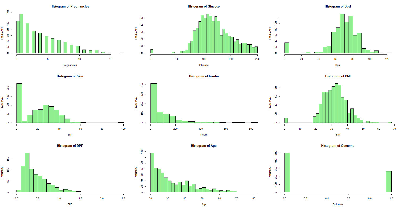
We observe that Glucose, Bpsi, Skin, Insulin, and BMI have minimum values of 0.0 in the dataset. This is clearly an impossible metric for these diagnostic measurements, so we must be dealing with missing data.
sum(dia$Glucose==0) / length(dia$Glucose) # proportion of missing glucose entries
sum(dia$Bpsi==0) / length(dia$Bpsi) # proportion of missing blood pressure entries
sum(dia$Skin==0) / length(dia$Skin) # proportion of missing skin thickness entries
sum(dia$Insulin==0) / length(dia$Insulin) # proportion of missing insulin entries
sum(dia$BMI==0) / length(dia$BMI) # proportion of missing body mass index entries
##  > sum(dia$Glucose==0) / length(dia$Glucose) # proportion of missing glucose entries
##  [1] 0.006510417
##  > sum(dia$Bpsi==0) / length(dia$Bpsi) # proportion of missing blood pressure entries
##  [1] 0.04557292
##  > sum(dia$Skin==0) / length(dia$Skin) # proportion of missing skin thickness entries
##  [1] 0.2955729
##  > sum(dia$Insulin==0) / length(dia$Insulin) # proportion of missing insulin entries
##  [1] 0.4869792
##  > sum(dia$BMI==0) / length(dia$BMI) # proportion of missing body mass index entries
##  [1] 0.01432292
Approximately 30% of SkinThickness values are missing as indicated by value 0. Similarly, nearly 49% of Insulin values are missing, 1% of Glucose values are missing, 5% of BloodPressure values are missing, and 1% of BMI values are missing from the data set. We will change the appropriate missing values to NA.
for (i in 1:768){
  for (j in 2:6){ # columns for Glucose, Bpsi, Skin, Insulin, BMI
    if (dia.df[i,j]==0){
      dia.df[i,j]=NA
    }
  }
}
Rather than working with patients who are missing diagnostic measurements, we will continue this analysis by only considering patients without missing values.
dia.df.subset = na.omit(dia.df)
dim(dia.df.subset)
## [1] 392 9
This subset only leaves us with 51% of the original entries. While this is not ideal, it allows for less data manipulation when constructing the final predictive model.
Next, we can create a Pearson correlation test matrix for this updated subset.
cor.dia.df.subset = cor(dia.df.subset) # correlation matrix for updated subset
diag(cor.dia.df.subset)=0
cor.dia.df.subset
##             Pregnancies   Glucose       Bpsi      Skin    Insulin         BMI          DPF        Age   Outcome
## Pregnancies  0.000000000 0.1982910  0.2133548 0.0932094 0.07898363 -0.02534728  0.007562116 0.67960847 0.2565660
## Glucose      0.198291043 0.0000000  0.2100266 0.1988558 0.58122301  0.20951592  0.140180180 0.34364150 0.5157027
## Bpsi         0.213354775 0.2100266  0.0000000 0.2325712 0.09851150  0.30440337 -0.015971104 0.30003895 0.1926733
## Skin         0.093209397 0.1988558  0.2325712 0.0000000 0.18219906  0.66435487  0.160498526 0.16776114 0.2559357
## Insulin      0.078983625 0.5812230  0.0985115 0.1821991 0.00000000  0.22639652  0.135905781 0.21708199 0.3014292
## BMI         -0.025347276 0.2095159  0.3044034 0.6643549 0.22639652  0.00000000  0.158771043 0.06981380 0.2701184
## DPF          0.007562116 0.1401802 -0.0159711 0.1604985 0.13590578  0.15877104  0.000000000 0.08502911 0.2093295
## Age          0.679608470 0.3436415  0.3000389 0.1677611 0.21708199  0.06981380  0.085029106 0.00000000 0.3508038
## Outcome      0.256565956 0.5157027  0.1926733 0.2559357 0.30142922  0.27011841  0.209329511 0.35080380 0.0000000
To better visualize this correlation matrix, we can use a heat map to plot the results
library(fields) # package for heat map
clockwise90 = function(a) { t(a[nrow(a):1,]) } # function to rotate heat map
image.plot(clockwise90(cor.dia.df.subset), col=heat.colors(12), axes=FALSE) # heat map of NA-removed correlations
par(cex.axis=.65)
axis(3, at=seq(0,1, length=9), labels=abbreviate(colnames(dia.df)), lwd=0, pos=1.1)
axis(2, at=seq(1,0, length=9), labels=abbreviate(colnames(dia.df)), lwd=0, pos=-0.1)
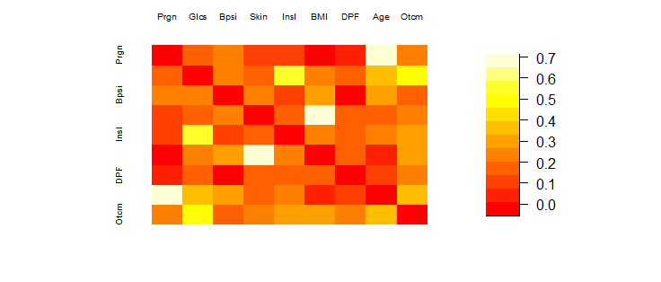
It appears that Age and Pregnancies have the largest correlation in the heat map. This makes sense as one might expect the number of pregnancies to increase as the age of a woman increases. However, this is not a correlation of interest. We are only focusing on variables that share a high correlation with Outcome of diabetes!
sorted.cor.subset = sort(cor.dia.df.subset, decreasing = TRUE)
sorted.cor.subset[1] # largest correlation
sorted.cor.subset[3] # second-largest correlation
sorted.cor.subset[5] # third-largest correlation
sorted.cor.subset[7] # fourth-largest correlation
## > sorted.cor.subset[1] # largest correlation
## [1] 0.6796085
## > sorted.cor.subset[3] # second-largest correlation
## [1] 0.6643549
## > sorted.cor.subset[5] # third-largest correlation
## [1] 0.581223
## > sorted.cor.subset[7] # fourth-largest correlation
## [1] 0.5157027
We can confirm that Age and Pregnancies did have the largest correlation of 0.67960847.
Skin and BMI place second with a correlation of 0.6643549.
Glucose and Insulin come in third place with a correlation of 0.581223.
Glucose and Outcome share a positive correlation of 0.5157027. This is a promising result! Intuition tells us that glucose level and the outcome of diabetes should share a positive correlation.
We can take another look at comparing the distributions of each field for those who have diabetes and those who do not. Each of the following box plots depict the distributions of each variable for patients who have diabetes (Outcome=1) and do not have diabetes (Outcome=0).
par(mfrow=c(2,4)) # Create plots for Outcome vs. Variables
for(j in 1:8){
plot(factor(dia.df.subset$Outcome), dia.df.subset[,j], main=paste("Outcome vs", colnames(dia.df.subset[j])), xlab="Outcome (0=no, 1=yes)", ylab=colnames(dia.df.subset[j]))
  }
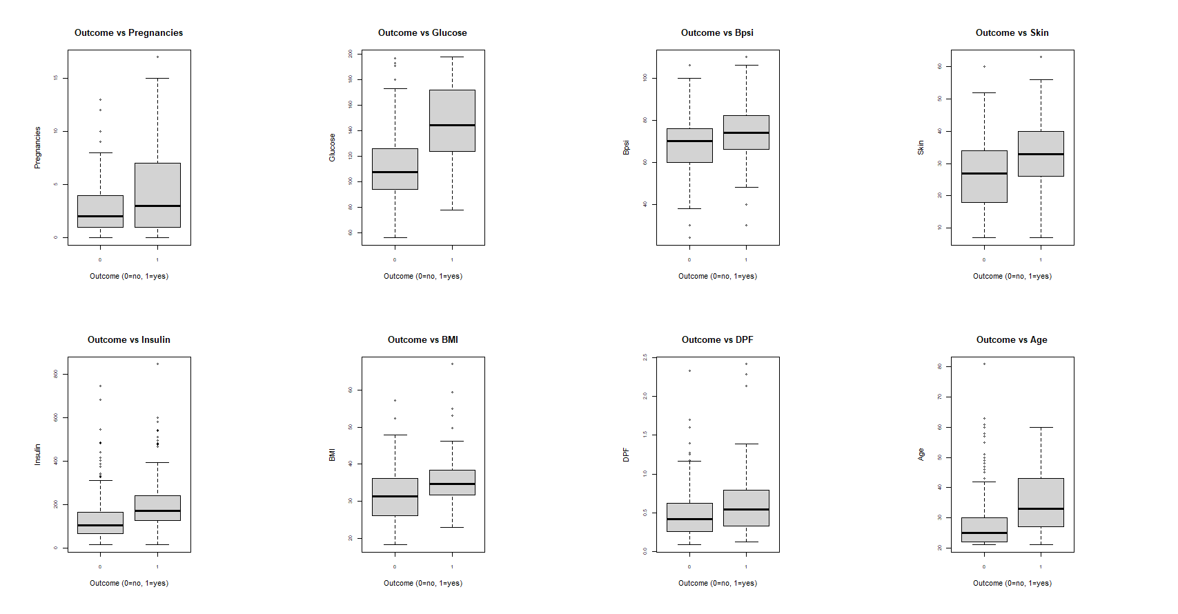
It can be seen again that Outcome and Glucose share some discrepancies. We can perform a t-test to see if there is a significant difference in the means of glucose for patients with and without diabetes.
t.test(dia.df.subset$Glucose[dia.df.subset$Outcome==0], dia.df.subset$Glucose[dia.df.subset$Outcome==1]) # t-test using data subset
##      Welch Two Sample t-test

## data:  dia.df.subset$Glucose[dia.df.subset$Outcome == 0] and dia.df.subset$Glucose[dia.df.subset$Outcome == 1]
## t = -11.151, df = 218.7, p-value < 2.2e-16
## alternative hypothesis: true difference in means is not equal to 0
## 95 percent confidence interval:
##  -39.72817 -27.79385
## sample estimates:
## mean of x mean of y
##  111.4313  145.1923
The t-test between Outcome and Glucose has a significant p-value (< 0.01). This indicates Glucose could be a reasonable variable to select in the final logistic regression model. The results when performing similar t-tests between Outcome and all remaining variables were also significant. Thus, we need to explore more criterion when selecting our model variables.
Backward selection is one common variable selection method when performing logistic regression. This method relies on the assessment of Akaike information criterion (AIC). AIC is a calculated model performance metric that estimates prediction error. We desire to minimize the AIC of our model for an optimal outcome. The method begins with all model variables selected. During each step of this procedure, we can choose to drop a single variable or stop. The deletion of each variable will alter the AIC of the model differently. This process ends when every remaining choice of variable deletion increases the model AIC. Here is an example of this selection method in R.
fit = glm(Outcome ~ ., data = dia.df.subset, family="binomial")

# Variable selection using Forward selection
stepwise = step(fit, direction = "backward")
summary(stepwise)
## Call:
## glm(formula = Outcome ~ Pregnancies + Glucose + BMI + DPF + Age,
##    family = "binomial", data = dia.df.subset)
##
## Coefficients:
##              Estimate Std. Error z value Pr(>|z|)
## (Intercept) -9.992080   1.086866  -9.193  < 2e-16 ***
## Pregnancies  0.083953   0.055031   1.526 0.127117
## Glucose      0.036458   0.004978   7.324 2.41e-13 ***
## BMI          0.078139   0.020605   3.792 0.000149 ***
## DPF          1.150913   0.424242   2.713 0.006670 **
## Age          0.034360   0.017810   1.929 0.053692 .
## ---
## Signif. codes:  0 ‘***’ 0.001 ‘**’ 0.01 ‘*’ 0.05 ‘.’ 0.1 ‘ ’ 1
##
## (Dispersion parameter for binomial family taken to be 1)
##
##     Null deviance: 498.10  on 391  degrees of freedom
## Residual deviance: 344.89  on 386  degrees of freedom
## AIC: 356.89
##
## Number of Fisher Scoring iterations: 5
The backward selection method chose to select the variables Insulin, BMI, DPF, and Age to predict Outcome. The model holds an AIC value of 356.89.
LASSO selection is another variable selection method used in logistic regression. LASSO stands for Least Absolute Shrinkage and Selection Operator and is an extension of ordinary least squares regression. The penalty imposed on the RSS is determined by multiplying a parameter λ with the sum of the absolute values of the non-intercept beta coefficients. This consequently increases the intensity of the penalty. Here is an example of this selection method in R.
library(glmnet)
x = model.matrix(Outcome~., data=dia)[,-1]
y = dia$Outcome
cv.lasso = cv.glmnet(x, y, family="binomial", alpha=1)
best.lambda = cv.lasso$lambda.min
best_model <- glmnet(x, y, family = "binomial", alpha = 1, lambda = best.lambda)
coef(best_model)
glm.res = glm(Outcome~Pregnancies+Glucose+Skin+BMI+DPF+Age, data = dia, family="binomial")
summary(glm.res)
## Call:
## glm(formula = Outcome ~ Pregnancies + Glucose + Skin + BMI +
##     DPF + Age, family = "binomial", data = dia)
##
## Coefficients:
##              Estimate Std. Error z value Pr(>|z|)
## (Intercept) -9.914004   1.090033  -9.095  < 2e-16 ***
## Pregnancies  0.083559   0.055160   1.515   0.1298
## Glucose      0.036485   0.004988   7.314 2.59e-13 ***
## Skin         0.011590   0.017058   0.679   0.4969
## BMI          0.067041   0.026122   2.566   0.0103 *
## DPF          1.130919   0.425725   2.656   0.0079 **
## Age          0.032892   0.017978   1.830   0.0673 .
## ---
## Signif. codes:  0 ‘***’ 0.001 ‘**’ 0.01 ‘*’ 0.05 ‘.’ 0.1 ‘ ’ 1
##
## (Dispersion parameter for binomial family taken to be 1)
##
##     Null deviance: 498.10  on 391  degrees of freedom
## Residual deviance: 344.42  on 385  degrees of freedom
## AIC: 358.42
##
## Number of Fisher Scoring iterations: 5
LASSO selects all variables except Bpsi and Insulin. This is similar to the backwards selection method with the addition of the variable Skin. Observe that this model holds an AIC value of 358.42, which is marginally worse than our previous model.
Exhaustive selection is another variable selection method for logistic regression. This procedure runs all possible regressions between the dependent variable and every possible subset of explanatory variables. This method is typically infeasible when dealing with many explanatory variables. However, since we are dealing with 9 total variables, we can afford this type of selection method.
library(bestglm)
library(leaps)
best.logit_AIC = bestglm(dia, IC = "AIC", family = binomial, method = "exhaustive")
best.logit_AIC$Subsets
##    Intercept Pregnancies Glucose  Bpsi  Skin Insulin   BMI   DPF   Age logLikelihood      AIC
## 0       TRUE       FALSE   FALSE FALSE FALSE   FALSE FALSE FALSE FALSE     -249.0489 498.0978
## 1       TRUE       FALSE    TRUE FALSE FALSE   FALSE FALSE FALSE FALSE     -193.3330 388.6660
## 2       TRUE       FALSE    TRUE FALSE FALSE   FALSE FALSE FALSE  TRUE     -185.3448 374.6897
## 3       TRUE       FALSE    TRUE FALSE FALSE   FALSE  TRUE FALSE  TRUE     -177.1828 360.3656
## 4       TRUE       FALSE    TRUE FALSE FALSE   FALSE  TRUE  TRUE  TRUE     -173.6175 355.2350
## 5*      TRUE        TRUE    TRUE FALSE FALSE   FALSE  TRUE  TRUE  TRUE     -172.4426 354.8851
## 6       TRUE        TRUE    TRUE FALSE  TRUE   FALSE  TRUE  TRUE  TRUE     -172.2121 356.4242
## 7       TRUE        TRUE    TRUE FALSE  TRUE    TRUE  TRUE  TRUE  TRUE     -172.0178 358.0356
## 8       TRUE        TRUE    TRUE  TRUE  TRUE    TRUE  TRUE  TRUE  TRUE     -172.0106 360.0212
Model 5 had the best AIC score selecting variables Pregnancies, Glucose, BMI, DPF, and Age. This selection of variables agrees with the backwards selection method. This model possesses the lowest possible AIC amongst all possible models with a value of 354.8851.
While there are many methods to consider while choosing variables for a logistic regression model, AIC and t-tests served as insightful and effective information criterion for this study.