Python: Simplex Algorithm Software
Background
Operations research is a broad field of study with connections to various subjects like linear algebra, graph theory, and combinatorics. Operations research is commonly associated with problems regarding optimization, such as the optimization of production schedules or resource allocation for a business. Many of these problems can be modeled using linear constraints and descriptive variables. Every problem has an objective function that is to be maximized or minimized. The simplex algorithm is a commonly used method when solving these types of linear programming (LP) problems. It requires that the original problem be written in a standard form with non-negative variables and linear constraints. An initial tableau or matrix can then be constructed for the algorithm to operate on. The algorithm itself runs a series of pivot operations on cells within each tableau iteration. Pivoting requires the performance of elementary row operations within the tableau to obtain a pivot cell. The simplex algorithm runs until there are no more appropriate cells to pivot, which will of course vary depending on the type of optimization and magnitude of the problem.
This software was programmed in Python using Replit. Public links to two versions of this software are posted on the UNC Charlotte Pages website for students in future operations research courses to use. This site can be found here.
Code
To begin programming an interactive simplex algorithm, the user must be prompted for inputs that record the dimensions of the initial tableau, the column (variable) names, and row entries (variable coefficients). Input-validation features are integrated throughout the program as well to ensure the algorithm will not crash from user errors. The user if first asked for the dimensions of the initial tableau.
import re

# Step 1: Get the dimensions of the initial tableau from the user
while True:
    try:
        num_rows = int(input("Enter the number of rows: "))
        num_cols = int(input("Enter the number of columns: "))
        break
    except ValueError:
        print("Invalid input. Please enter an integer value.")
Next, the user is prompted to input the column names of the initial tableau. These names represent the variables that are used in the standardized linear programming problem. Column names in this input are to be separated by spaces.
# Step 2: Get the column names from the user
while True:
    col_names = input("Enter the column names separated by spaces: ").split()
    if len(col_names) == num_cols:
        break
    else:
        print(f"Invalid input. Expected {num_cols} column names separated by spaces.")
Similarly, the user must enter the entries for each row in the initial tableau. Provided any matrix with m rows and n columns, the user must enter exactly n values for m distinct rows. Entries in each row are separated by spaces, and rows are separated by semicolons.
# Step 3: Create the initial tableau with user input values
matrix = []
while True:
    matrix_input = input(f"Enter values for the matrix of size {num_rows}x{num_cols}, separating rows by semicolons (;): ")
    matrix_rows = matrix_input.strip().split(';')
    if len(matrix_rows) != num_rows:
        print(f"Invalid input. Please enter {num_rows} rows separated by semicolons.")
        continue
    matrix_cols = [row.strip().split() for row in matrix_rows]
    valid_input = True
    for row in matrix_cols:
        if len(row) != num_cols:
            valid_input = False
            print(f"Invalid input. Please enter {num_cols} values per row.")
            break
        try:
            row = [float(val) for val in row]
        except ValueError:
            valid_input = False
            print("Invalid input. Please enter numerical values only.")
            break
    if valid_input:
        matrix = [[float(val) for val in row] for row in matrix_cols]
        break
Once the initial tableau is properly entered, it can be displayed back to the user.
# Step 4: Display the initial tableau with centered column names
print("Initial tableau:")
for col_name in col_names:
    print(f"{col_name:^10}", end="")
print()
for row in matrix:
    for val in row:
        if val >= 0:
            print(f"{val:^10.3f}", end="")
        else:
            print(f"{val:^11.3f}", end="")
    print()
Next, the program prompts the user for the coordinates of the first pivot cell. Determining which cell to pivot requires some background knowledge in linear programing. Pivots are chosen differently depending on whether the problem is a maximization or minimization problem. If the initial problem is a maximization problem, the algorithm will scan the first row of the tableau (representative of the objective function) to locate the greatest negative value. This determines the pivot column. The pivot column (excluding the value in the first row) is used in a ratio test with the last column on the “right-hand side” of the tableau. In these rows, the right-hand side value is divided by the value found in the pivot column. If a value is negative or zero and belongs to the pivot column, it is not included in the ratio test. The smallest ratio determines the pivot row. Intuitively, the pivot cell can be located at the intersection of the pivot row and column.
A minimization problem shares a similar procedure, finding the greatest positive value in the first row and performing ratio tests with negative values. Of course, some technicalities can alter these rules, but this is the general method of the simplex algorithm. Once a cell is pivoted, the algorithm repeats this process until there are no more available pivot columns.
# Step 5: Get the cell to pivot from the user
while True:
    pivot_input = input("Enter the coordinates of the cell to pivot (x,y): ")
    pivot_coords = re.findall(r'\d+', pivot_input)
    if len(pivot_coords) == 2:
        pivot_row, pivot_col = int(pivot_coords[0]), int(pivot_coords[1])
        if 1 <= pivot_row <= num_rows and 1 <= pivot_col <= num_cols:
            break
    print("Invalid input. Please enter the coordinates in the format (x,y) where x is the row number and y is the column number.")
Here is the pivot function.
# Step 6: Perform the pivot function to make the cell pivoted
pivot_val = matrix[pivot_row-1][pivot_col-1]
for i in range(num_cols):
    matrix[pivot_row-1][i] /= pivot_val
for i in range(num_rows):
    if i != pivot_row-1:
        multiplier = matrix[i][pivot_col-1]
        for j in range(num_cols):
            matrix[i][j] -= multiplier * matrix[pivot_row-1][j]
After each pivot, the updated tableau is displayed to the user.
# Step 7: Display the updated tableau after pivoting
print()
print("After pivoting:")
for col_name in col_names:
    print(f"{col_name:^10}", end="")
print()
for row in matrix:
    for val in row:
        print(f"{val:^10.3f}", end="")
    print()
Finally, the algorithm repeats after its first iteration.
# Step 8: Get the next cell to pivot from the user
while True:
    pivot_input = input("Enter the coordinates of the next cell to pivot (x,y): ")
    pivot_coords = re.findall(r'\d+', pivot_input)
    if len(pivot_coords) == 2:
        pivot_row, pivot_col = int(pivot_coords[0]), int(pivot_coords[1])
        if 1 <= pivot_row <= num_rows and 1 <= pivot_col <= num_cols:
            # Check if the cell to pivot has a value of 0
            if matrix[pivot_row-1][pivot_col-1] == 0:
                print("Cannot pivot a cell with value 0. Please enter the coordinates of another cell.")
                continue

            # Perform the pivot function to make the cell pivoted
            pivot_val = matrix[pivot_row-1][pivot_col-1]
            for i in range(num_cols):
                matrix[pivot_row-1][i] /= pivot_val
            for i in range(num_rows):
                if i != pivot_row-1:
                    multiplier = matrix[i][pivot_col-1]
                    for j in range(num_cols):
                        matrix[i][j] -= multiplier * matrix[pivot_row-1][j]

            # Display the updated tableau after pivoting
            print()
            print("After pivoting:")
            for col_name in col_names:
                print(f"{col_name:^10}", end="")
            print()
            for row in matrix:
                for val in row:
                    print(f"{val:^10.3f}", end="")
                print()

        else:
            print(f"Invalid input. Please enter a cell within the tableau dimensions (1-{num_rows}, 1-{num_cols}).")
    else:
        print("Invalid input. Please enter the coordinates in the format (x,y) where x is the row number and y is the column number.")
Demonstration
The following example is a popular linear programming problem from the online textbook Operations Research for Electrical Engineering.
The Dakota Furniture Company manufactures desks, tables, and chairs. The manufacture of each type of furniture requires lumber and two types of skilled labor: finishing and carpentry.
- A desk requires 8 board feet of lumber, 4 finishing hours, and 8 carpentry hours.
- A table requires 6 board feet of lumber, 2 finishing hours, and 1.5 carpentry hours.
- A chair requires 1 board foot of lumber, 1.5 finishing hours, and 0.5 carpentry hours.
Currently, 48 board feet of lumber, 20 finishing hours, and 8 carpentry hours are available. A desk sells for $60, a table for $30, and a chair for $20. Dakota believes that demand for desks and chairs is unlimited, but at most five tables can be sold. Because the available resources have already been purchased, Dakota wants to maximize total revenue.
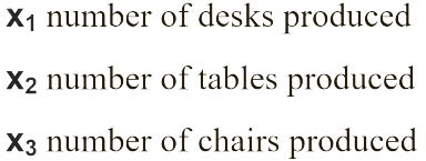
Define the decision variables as:

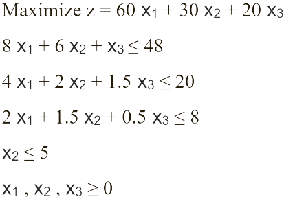
This problem can be modeled by the following LP:

This is a standard maximization linear programing problem. To convert this problem into standard form, inequalities must be changed to equalities by introducing non-negative slack variables in each constraint. Additionally, the right-hand side of the objective function must hold a value of zero, which can be achieved using simple algebra. Once the problem is in standard form, it can be written as an initial tableau.

Now that the initial tableau is obtained, the simplex algorithm program can be utilized to solve this problem.

The program now calls for the coordinates of the first pivot cell. This problem is a standard maximization LP, so the pivot column is determined by the greatest negative value in the first row. -60 is the correct choice, so column two be the pivot column. Next, a ratio test is performed to determine the pivot cell.
48/8 = 6
20/4 = 5
8/2 = 4
Recall that zero-entries are not included in the ratio test. 4 is the smallest ratio, so row 4 is the pivot row. Thus, the first pivot cell has the coordinates (4,2).

By pivoting this cell, the desks variable x1 corresponding to the pivot column becomes a basic variable. In a basic variable column, the pivoted cell holds a value of 1 while the remaining cells hold a value of 0. The program calculates this result by performing elementary row operations amongst the pivot and non-pivot rows. All basic variables hold value in a basic feasible solution. A basic feasible solution to an LP is a solution that meets the requirements of each constraint. However, not all basic feasible solutions are optimal. This second tableau is a basic feasible solution that suggests 4 desks be produced for a profit of $240. However, this is not an optimal solution because there is another cell to pivot in the updated tableau. The next pivot cell has the coordinates (3,4).

After this pivot, the chairs variable x3 becomes a basic variable. This new basic feasible solution suggests producing 2 desks and 8 chairs for a profit of $280. Since there are no more negative values in the first row of the updated tableau, the optimal solution has been reached. Therefore, the company should produce 2 desks and 8 chairs to maximize their total revenue based on the given constraints.
