
R: Differential Expression of Genes in PDAC Tumor Samples
Background
The purpose of this project was to identify differentially expressed genes from an over-dispersed count data set comprised of 148 PDAC tumor samples. Each tumor sample held a neoplastic cellularity percentage and count values corresponding to one of 17394 genes per sample. This project began with an analysis of the Poisson and negative binomial distributions (two common distributions used to model count data) and their effectiveness in modeling count data exhibiting overdispersion. It was determined that neither of these distributions could meet the desired accuracy of modeling this PDAC data set. Normal Quantile-Quantile plots were also constructed to visualize these inaccuracies. The Poisson-Tweedie distribution (from the ‘tweedie’ CRAN R package) demonstrated suitability in modeling the PDAC data set after conducting 12000+ simulated experiments testing the goodness-of-fit of estimated model parameters on over-dispersed data. An additional series of simulation studies were performed to test the empirical power of a differential-expression-test function on distinct Poisson-Tweedie distributions. This function proved to be powerful and effective in detecting differential expression between subsets in the PDAC data set. The PDAC data was split into two subsets for the first analysis. All tumor samples with low neoplastic cellularity levels (less than 0.5) were assigned to group A. The remaining tumor samples with high neoplastic cellularity levels (greater than or equal to 0.5) were assigned to group B. The second analysis focused on the explicit neoplastic cellularity values of each tumor sample. Linear regression modeling was performed on both analyses to successfully detect 1403 consensus genes from the original data supporting known prognostic markers in human cancer.
Description
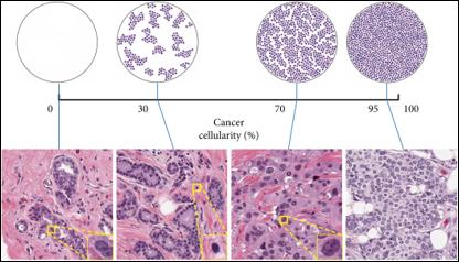
Pancreatic Ductal Adenocarcinoma (often referred to as PDAC) is a type of pancreatic cancer that is the 4th leading cause of cancer-related deaths around the world today. This disease is projected to become the 2nd leading cause of cancer deaths by 2030. There are several challenges in treating PDAC. Due to the lack of effective treatment options, the median survival of PDAC is 6 months, and the 5-year survival rate is less than 10% after diagnosis. Neoplastic cellularity is the term used to define the proportion of cancerous cells to healthy cells within a bulk tumor sample. PDAC tumor samples tend to have low neoplastic cellularity, meaning they are comprised of significantly fewer cancerous cells than normal cells.
With a lack of screening biomarkers for PDAC, this low neoplastic cellularity in tumor samples makes the disease difficult to diagnose in its early stages. The goal of this study is to identify the presence of differentially expressed (DE) genes between the healthy and cancerous cells that make up PDAC tumor samples.
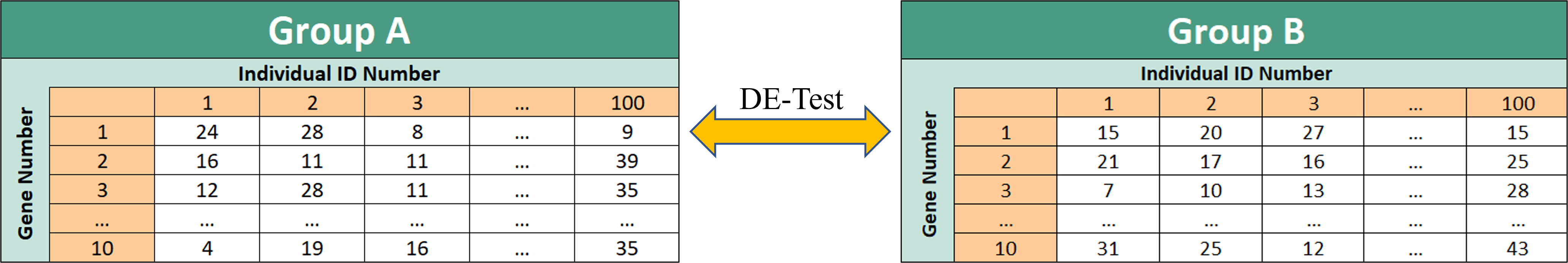
Modeling gene expression for this study requires a probability model that can measure genetic count data from PDAC tumor samples. The following table depicts a simple example of how the count data is formatted. Both the Poisson and Negative Binomial distributions are two common count-data probability models that were initially considered. It is important to note the presence of overdispersion in certain data sets. Overdispersion is a property that occurs in a data set when the variance of the data is greater than the expected value of the data, denoted as µ. This particular study of DE genes requires a probability distribution that can model over-dispersed count data. When considering the Poisson model, it was important to recognize the expected value of the distribution is always equal to the variance of the distribution. Therefore, a Poisson model cannot account for overdispersion in a count data set, and thus was not the best choice to model the data. The Negative Binomial model, on the other hand, has the ability to model overdispersion in count data. However, it is still rare for a Negative Binomial distribution to model a count data set with the desired accuracy for this study. The Poisson-Tweedie (PT) model utilizes more parameters than both previous distributions and consequently offers more accuracy in modeling an over-dispersed count data set. These parameters include µ, the expected value; D, the dispersion index; and α, the shape parameter of the distribution. By modifying the shape parameter α, a PT model can mimic both the Poisson and Negative Binomial distributions, providing the most flexible model for this data study (this will also be seen in the following slides). Multiple simulation studies were conducted to further analyze the benefits of using the PT model.
Simulation Testing
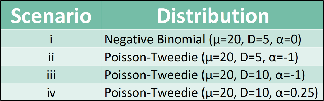
Four simulation studies were conducted to evaluate estimated PT distribution parameters. These simulations tested the accuracy of a PT-parameter estimating function. Each scenario was tested using 3 different sample sizes (100, 200, and 500). This was done to investigate the effectiveness of the function when increasing the sample size of the simulated data.
Here is a standard procedure for conducting the simulations in Scenario II when sample size n=200:
# rtweedie Scenario II

library(tweedie)
library(tweeDEseq)
set.seed(123)
mu.res <- d.res <- a.res <- NB.pvalues <- Pois.pvalues <- c(1:1000) #Create five vectors of size 1000

for (i in 1:1000){

y <- rPT(n=200, mu=20, D=5, a=-1)
thetahat <- mlePoissonTweedie(y)

mu.res[i] <- getParam(thetahat)[1]
d.res[i] <- getParam(thetahat)[2]
a.res [i] <- getParam(thetahat)[3]


# Test fit to Negative Binomial Distribution
NB.pval <- testShapePT(thetahat, a=0)
NB.pvalues[i] <- NB.pval$pvalue

# Test fit to Poisson Distribution
Pois.pval <- testShapePT(thetahat, a=1)
Pois.pvalues[i] <- Pois.pval$pvalue


}

mean(mu.res) #Average mu value
mean(d.res) #Average D value
mean(a.res) #Average a value

NB.pvalues <- sort(NB.pvalues, decreasing = FALSE) #Sorts P-values from lowest to highst
which(NB.pvalues<0.05) #Lists indicies of significant p.values lower than 0.05

Pois.pvalues <- sort(Pois.pvalues, decreasing = FALSE) #Sorts P-values from lowest to highst
which(Pois.pvalues<0.05) #Lists indicies of significant p.values lower than 0.05

hist(mu.res)
hist(d.res)
hist(a.res)
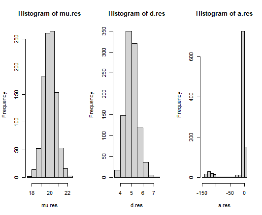
We see that the estimated shape parameters in each histogram are normally distributed with a mean value close to the true parameter value of these simulated Poisson-Tweedie distributions. It is worth noting the cluster of outliers in the alpha parameter histogram. By repeating similar simulations that meet the sample size requirements for each scenario, we obtain the following visual:
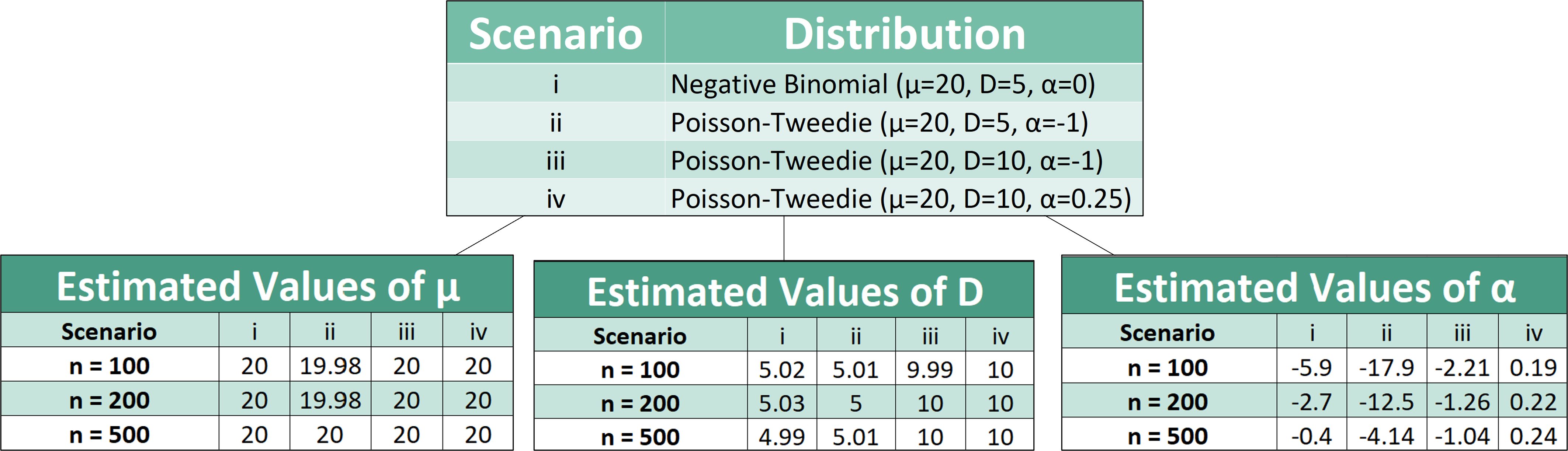
The results show that the PT-parameter estimating function provides good estimates of the PT parameters µ and D regardless of sample size. As for the PT parameter α, increasing the sample size of the simulated data improved the parameter estimates.
The same four simulated scenarios were also used to test the empirical power of the PT-goodness-of-fit function. These simulations tested whether or not a particular scenario’s distribution shape deviated from that of the Negative Binomial or Poisson distribution. The shape of each distribution from the four scenarios were compared to the Negative Binomial and Poisson distributions holding PT parameter values α=0 and α=1, respectively. This shape test was performed on each of the 1000 replicates for every simulation. The following 2-sided hypothesis test was performed to detect the number of distributions out-of-1000 that rejected the null hypothesis (H0: α=0 for Negative Binomial test or H0: α=1 for Poisson test). In other words, how many distributions had shapes that were deemed significantly different from the shape of a Negative Binomial or Poisson distribution. Here is an example of how both tests were performed in Scenario II with sample size n=200:
library(tweeDEseq)
set.seed(123)
mu.res <- d.res <- a.res <- NB.pvalues <- Pois.pvalues <- c(1:1000) #Create five vectors of size 1000

for (i in 1 : 1000)
{
  y <- rnbinom(n=200, size=5, p=0.2)
  thetahat <- mlePoissonTweedie(y)

  mu.res[i] <- getParam(thetahat)[1]
  d.res[i] <- getParam(thetahat)[2]
  a.res [i] <- getParam(thetahat)[3]

  # Test fit to Negative Binomial Distribution
  NB.pval <- testShapePT(thetahat, a=0)
  NB.pvalues[i] <- NB.pval$pvalue

  # Test fit to Poisson Distribution
  Pois.pval <- testShapePT(thetahat, a=1)
  Pois.pvalues[i] <- Pois.pval$pvalue
}

length(which(NB.pvalues<0.05)) # total significant tests for the Negative Binomial distribution
length(which(Pois.pvalues<0.05)) # total significant tests for the Negative Binomial distribution
Similar tests were performed for the remaining scenarios and sample sizes. This visual depicts the results of these simulations:
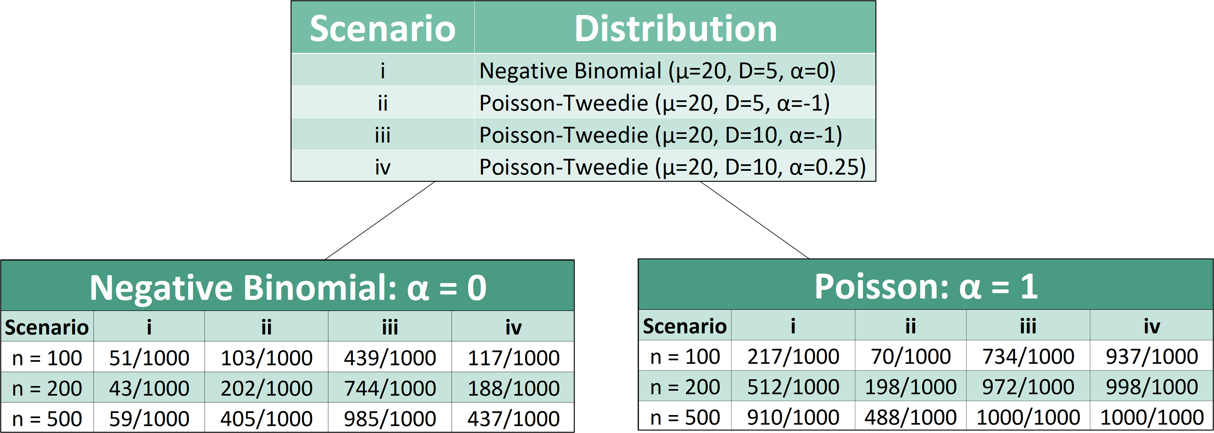
One can conclude from the following simulated tests that the type one error rate (0.05) is well maintained around the nominal level when comparing two negative binomial distributions to one another (as seen in scenario one). Further deviation from the null scenario (such as scenario 3) shows the highest empirical power for the test. Additionally, the power of this goodness-of-fit function improves as sample size increases.
Another set of simulation studies were conducted to test the empirical power of the DE-testing function by strategically modifying parameters µ and D. The DE-testing function tests the following null hypothesis to determine whether or not 2 PT distributions share the same parameter value µ. This 2-sided hypothesis test was performed on the following 18 simulations to detect the number of distributions out of 1000 replicates that rejected this null hypothesis. 9 simulated tests were performed on the Negative Binomial distribution (where a=0) and 9 additional tests were performed on the Pólya distribution (where a=-1). The following example shows how each of the 18 tests were performed to test the DE-detection capability of this function for two different PT distributions. For each simulation, two count-data groups were assigned 1000 read counts. These read counts were then sorted to represent the count data of 10 different genes for 100 individuals. A DE-test was then performed between the two groups and replicated 1000 times.
Here is an example of how these simulations were executed. Note that parameters were properly adjusted to fit the requirements for each simulated trial in the final visual:
library(tweeDEseq)
set.seed(123)
n=100 # number of individuals in each group
pvalues <- c()

for (i in 1 : 10)
{
  counts_0 <- matrix(rPT(n = 1000, a = 0.5, mu = 20, D = 5), ncol = 100) # generate read counts data for 10 genes in the first group
  counts_1 <- matrix(rPT(n=1000, a=0.5, mu=20, D=5), ncol=100) # generate read counts data for 10 genes in the second group.
  counts <- cbind(counts_0, counts_1) # combine them together
  G <- rep(c(1,2), each=100) # generate group label.
  # Test for differences between the two groups
 DE.res <- tweeDE(counts, group = G) # test
  pvalues <- rbind(pvalues, DE.res$pval.adjust)
}
The 2 following bar plots show the average DE detection rate when the DE-test was performed in 9 trials for both tables.
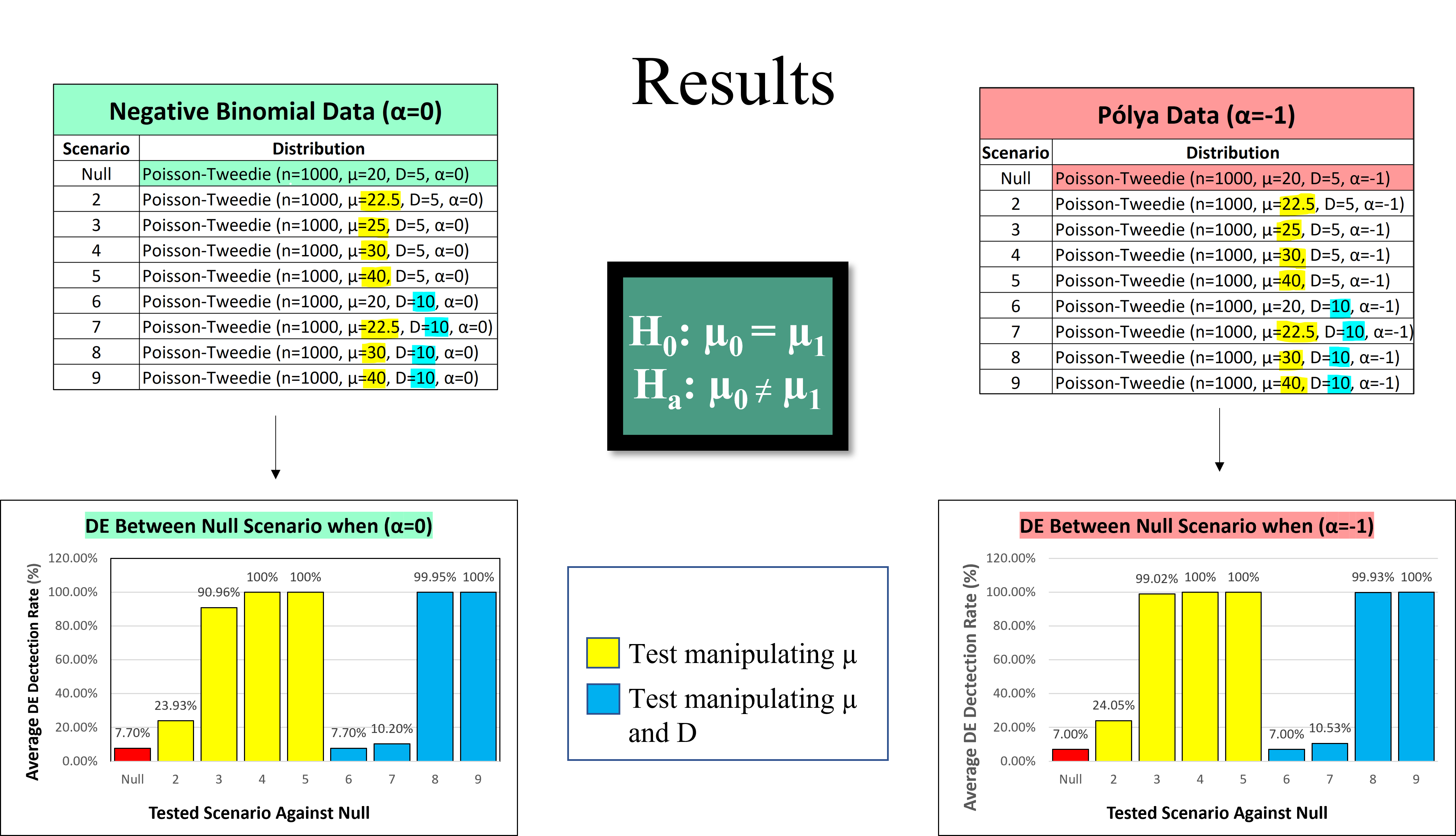
This set of simulations demonstrated that the proportion of tests rejecting the Null Hypothesis increases as the parameter difference grows further apart for both parameters µ and D. This was the case for all simulated data sets from both the Negative Binomial and Pólya distributions. Again, the type one error rate (0.05) is well maintained around the nominal level when comparing two PT distributions with equivalent µ values (as seen in both Null vs. Null scenarios). Larger D parameter values lead to a moderately inflated type one error rate which slightly lowered the test’s empirical power. However, it was concluded that the DE-testing function was efficient on different PT distributions as well as its practicality on real data sets varying from a Negative Binomial shape.
Real Data Analysis
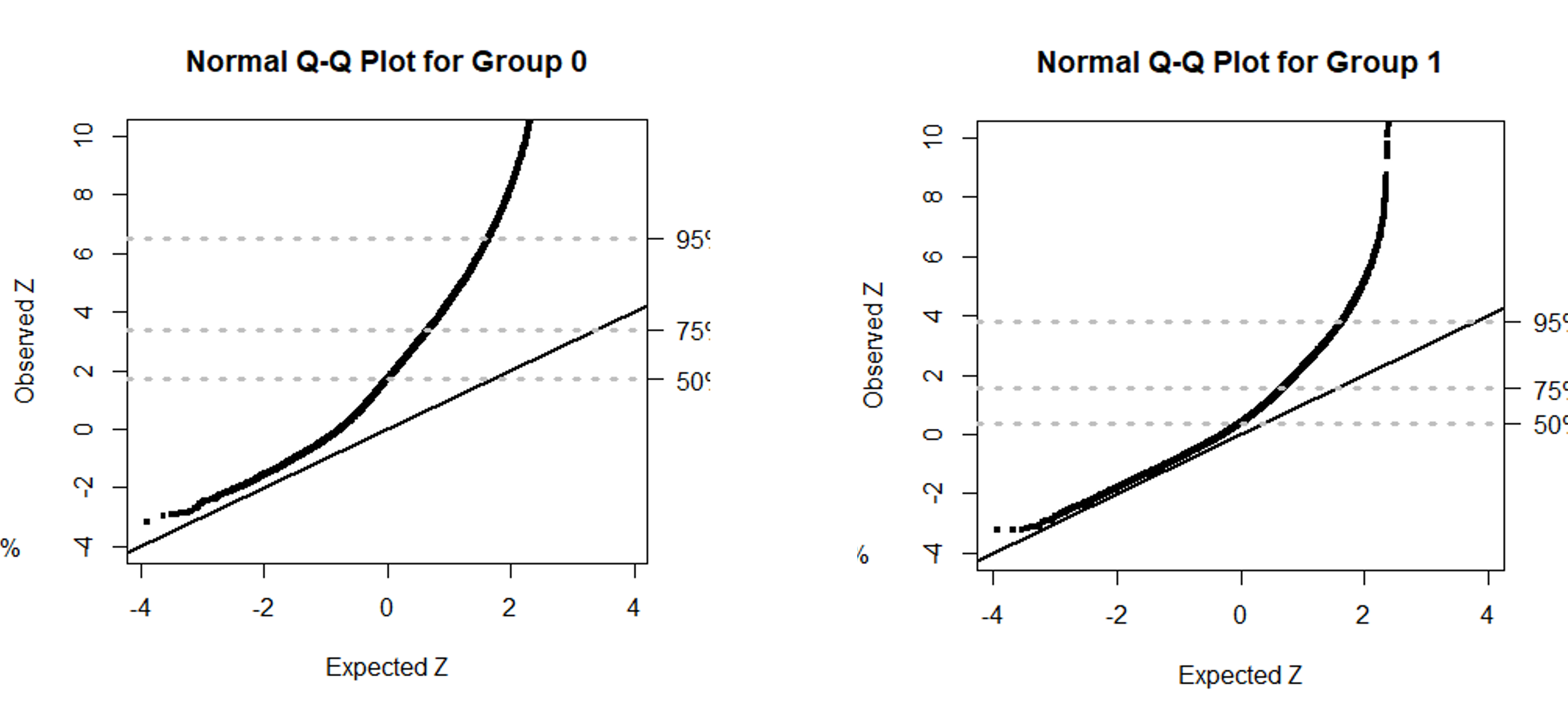
For the real PDAC data analysis, all the data was downloaded from The Cancer Genome Atlas (TCGA) Project. This data was made up of 148 PDAC tumor samples consisting of 17,394 genes per sample. Each tumor sample was also labeled with neoplastic cellularity. From there, each tumor sample was sorted into one-of-two groups based on its neoplastic cellularity. Samples placed in Group 0 had purity levels less than 50%, while samples placed in Group 1 had purity levels greater than or equal to 50%. After sorting the tumor samples, a goodness-of-fit test was used to test the fit of both groups to a Negative Binomial function producing the following quantile-quantile plots. Both plots depict chi-square statistics as standard normal scores that assess the goodness-of-fit between group data and the Negative Binomial model. The genes in both groups have expression profiles that deviate significantly from the Negative binomial model. Therefore, an alternative distribution (like the PT distribution) should be used to accurately model this count data.
library(readr)
clinic <- read_csv("UNCC/2021-2022 Research/PAAD_clinic.csv")
RNAdata = read.table("UNCC/2021-2022 Research/PAAD_RNAseq.txt")

group0 <- which(clinic$paper_ABSOLUTE.Purity < 0.5) # Minority group
group1 <- which(clinic$paper_ABSOLUTE.Purity >= 0.5) # Majority group

sortedG0 <- RNAdata[group0] #Ordered group0 data
sortedG1 <- RNAdata[group1] #Ordered group1 data

#Goodness-of-fit
gof0 <- gofTest(sortedG0, a=0)
gof1 <- gofTest(sortedG1, a=0)

chi0 <- qqchisq(gof0, main="Chi2 Q-Q Plot for Group 0", ylim = c(0, 2000)) #Chi2 Q-Q Plot
norm0 <- qqchisq(gof0, normal=TRUE, main="Normal Q-Q Plot for Group 0", ylim = c(-4, 10)) #Normal Q-Q Plot

chi1 <- qqchisq(gof1, main="Chi2 Q-Q Plot for Group 1", ylim = c(0, 2000)) #Chi2 Q-Q Plot
norm1 <- qqchisq(gof1, normal=TRUE, main="Normal Q-Q Plot for Group 1", ylim = c(-4, 10)) #Normal Q-Q Plot
Two analyses were conducted on the PDAC count data set to detect DE genes using the following statistical model. The expression level 𝑌𝑖𝑔 of a given gene (𝑔) in a sample (𝑖) follows the following PT distribution: 𝑌𝑖𝑔~𝑃𝑇(𝜇𝑔,𝐷𝑔,α𝑔)
Similarly, let 𝑥𝑖𝑐 and 𝑥𝑖𝑛 denote the proportion of cancerous and normal cells in a given sample.
Primary linear regression model: log(𝜇𝑔)=𝛽0+𝛽1𝑥𝑖𝑐
The first analysis was conducted by the previous DE-testing function between Group 0 and Group 1 based on neoplastic cellularity. Here, all neoplastic cellularity values are possible inputs for 𝑥𝑖𝑐.
The second analysis of the data used a linear regression model to test for differential expression strictly based on a gene’s neoplastic cellularity level being above 50%. This type of binary approach only allowed for the values 0 or 1 as functional inputs for 𝑥𝑖𝑐.
A DE test was then performed on the genes by determining H0: 𝛽1=0 vs. Ha:𝛽1≠0 in either analysis.
library(tweeDEseq)
counts <- cbind(sortedG0, sortedG1) #DE Analysis
G <- rep(0,148)
G[108:148] <- 1
DE.res <- tweeDE(counts, group = G)

par(mfrow(c(1,2)))
hist(DE.res$pval.adjust, breaks = seq(0,1,.01), main="Histogram of Adjusted P-values", xlab="Adjusted P-Value") #Histogram of adjusted P-values
hist(DE.res$log2fc, main="Histogram of log2 Fold-Change", xlab="log2 Fold-Change", breaks=96, xaxp=c(-3,3,12)) #Histogram of fold change
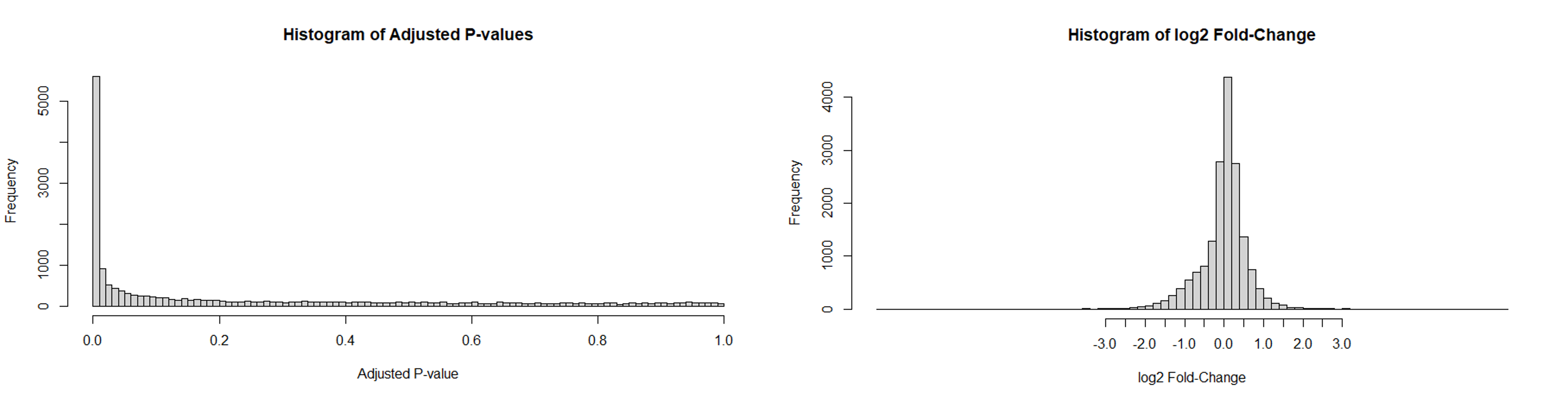
From the first analysis, a histogram of the adjusted P-values from the DE test depicts a spike of significant P-values (less than 0.05) indicating a surplus of DE genes that were detected between both groups. A histogram of the log2 fold-change from the DE test shows several genes fall beyond a cutoff point of 1.5. This indicates the presence of over-dispersed genes in the data set. These over-dispersed genes have a significant difference in quantity between both groups.
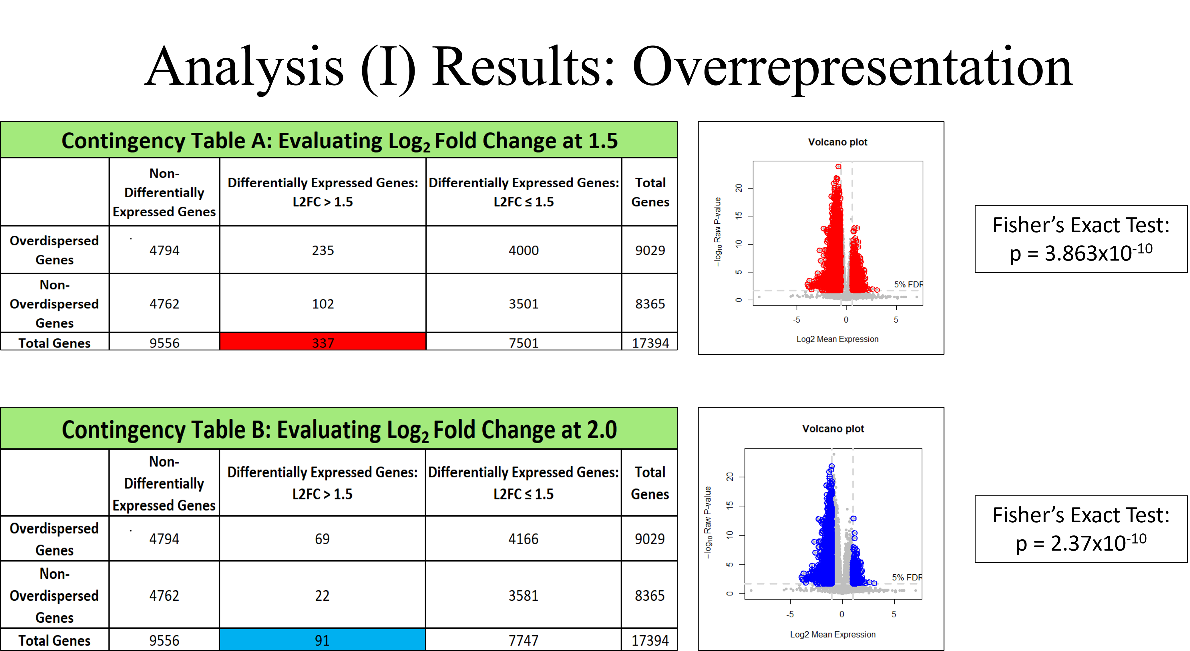
In this analysis, an overrepresented gene is said to have passed the DE-test with a p-value less than 0.05 and exceeds a log2 fold-change of 1.5 between the low and high neoplastic cellularity groups. Note that by increasing the log2 fold-change cutoff value, the number of overrepresented genes decreases. The following volcano plots depict these overrepresented genes using two different log2 fold-change cutoff values. Fisher’s exact test was performed on both contingency tables and returned significant P-values. This confirmed the presence of overrepresented genes in the data set.
deGenesA <- rownames(print(DE.res, n=Inf, log2fc=log2(1.5), pval.adjust=0.05, print=FALSE))
deGenesB <-  rownames(print(DE.res, n=Inf, log2fc=log2(2.0), pval.adjust=0.05, print=FALSE))
deGenesC <-  rownames(print(DE.res, n=Inf, log2fc=log2(2.5), pval.adjust=0.05, print=FALSE))

# Goodness-of-fit
gof0 <- gofTest(sortedG0, a=0)
gof1 <- gofTest(sortedG1, a=0)

chi0 <- qqchisq(gof0, main="Chi2 Q-Q Plot for Group 0", ylim = c(0, 2000)) #Chi2 Q-Q Plot
norm0 <- qqchisq(gof0, normal=TRUE, main="Normal Q-Q Plot for Group 0", ylim = c(-4, 10)) #Normal Q-Q Plot

chi1 <- qqchisq(gof1, main="Chi2 Q-Q Plot for Group 1", ylim = c(0, 2000)) #Chi2 Q-Q Plot
norm1 <- qqchisq(gof1, normal=TRUE, main="Normal Q-Q Plot for Group 1", ylim = c(-4, 10)) #Normal Q-Q Plot

# Volcano Plot(s)
hl <- list(genes=deGenesA, pch=1, col="red", lwd=2, cex=1.5)
Vplot(DE.res, cex=0.7, highlight=hl, log2fc.cutoff=log2(1.5), pval.adjust.cutoff=0.05, main="Volcano plot", xlab="Log2 Mean Expression")
---------------------------
# Contingency Table
Pf0 <- -pchisq(gof0, df=1, lower.tail=FALSE)
Pf1 <- -pchisq(gof1, df=1, lower.tail=FALSE)
overdispersed <- names(gof0)[Pf0 < 0.05 & Pf1 < 0.05 & !is.na(Pf0) & !is.na(Pf1)]

allGenes <- rownames(counts) # List of all gene names

nonDEG <- which(DE.res$pval.adjust >= 0.05) # Indices of all non-DE genes

# Log2FoldChange = 1.5 Table
bigFoldA <- which(abs(DE.res$log2fc) > 1.5 & DE.res$pval.adjust < 0.05) # Indices of DE genes with fold > 1.5
smallFoldA <- which(abs(DE.res$log2fc) < 1.5 & DE.res$pval.adjust < 0.05) # Indices of DE genes with fold <= 1.5

length(intersect(overdispersed, allGenes[nonDEG])) # non-DE and overdispersed
length(intersect(overdispersed, allGenes[bigFoldA])) # DE and Fold > 1.5, overdispersed
length(intersect(overdispersed, allGenes[smallFoldA])) # DE and Fold <= 1.5, overdispersed
---------------------------
# Log2FoldChange = 2.0 Table
bigFoldB <- which(abs(DE.res$log2fc) > 2.0 & DE.res$pval.adjust < 0.05) # Indices of DE genes with fold > 2.0
smallFoldB <- which(abs(DE.res$log2fc) < 2.0 & DE.res$pval.adjust < 0.05) # Indices of DE genes with fold <= 2.0

length(intersect(overdispersed, allGenes[nonDEG])) # non-DE and overdispersed
length(intersect(overdispersed, allGenes[bigFoldB])) # DE and Fold > 2.0, overdispersed
length(intersect(overdispersed, allGenes[smallFoldB])) # DE and Fold <= 2.0, overdispersed
Consensus DE genes were discovered by identifying which genes were detected in both sets of analyses. These 1403 consensus genes are the most likely to express true differential expression. Identified genes that were not consensus DE genes may suggest true DE genes OR other marker genes due to neoplastic cellularity.
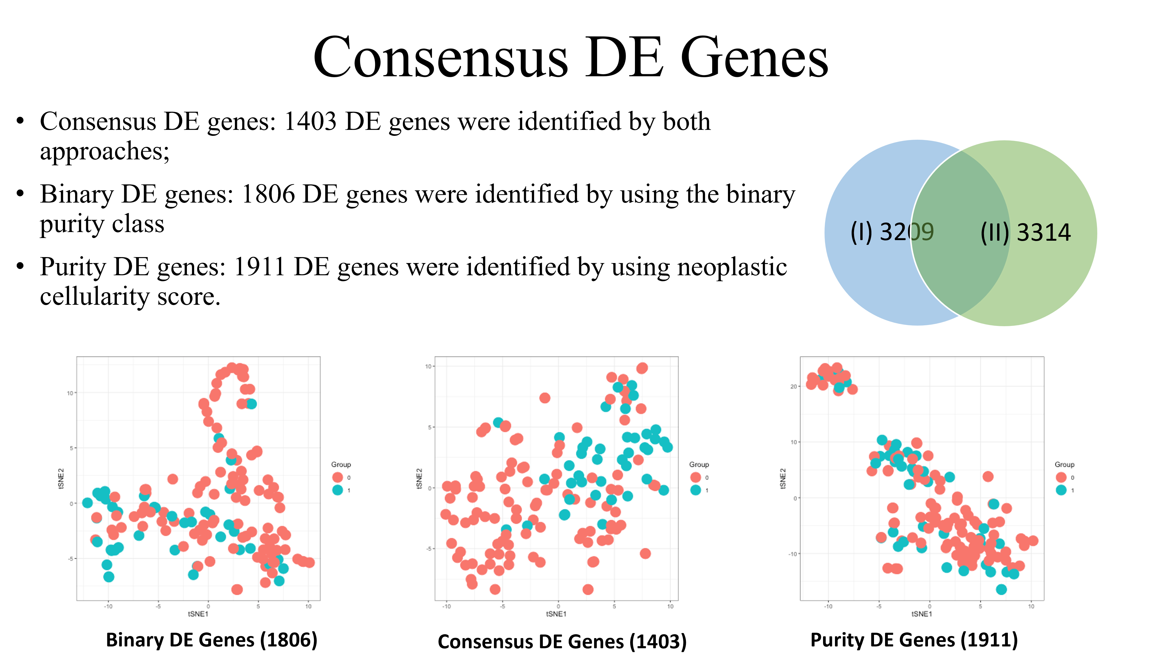
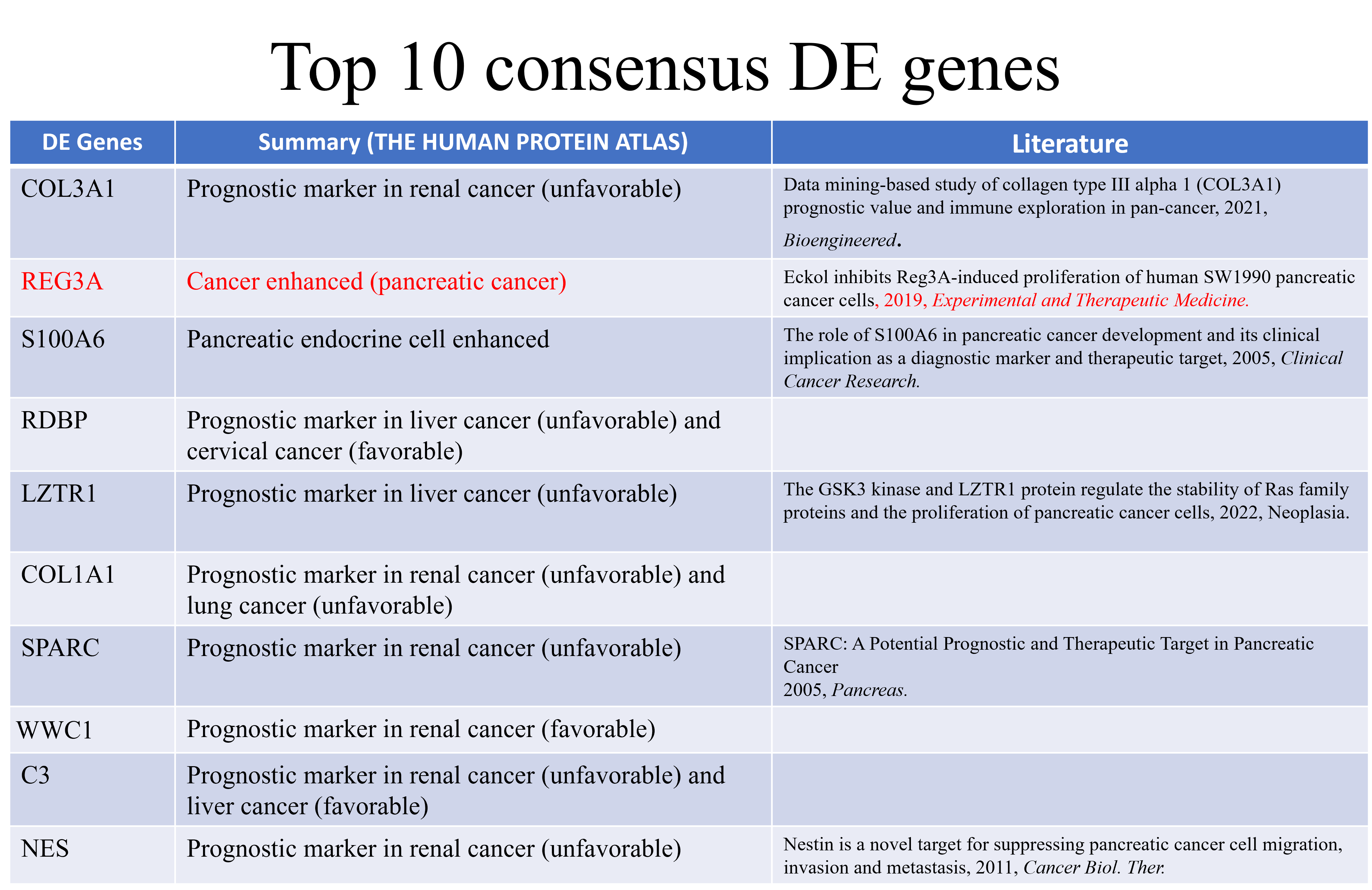
Here, the top 10 consensus DE genes are recorded. It is important to note that the majority of these consensus DE genes have already been determined as prognostic markers in human cancer. To name one example, one literary report previously associated the consensus DE gene COL3A1 with PDAC.
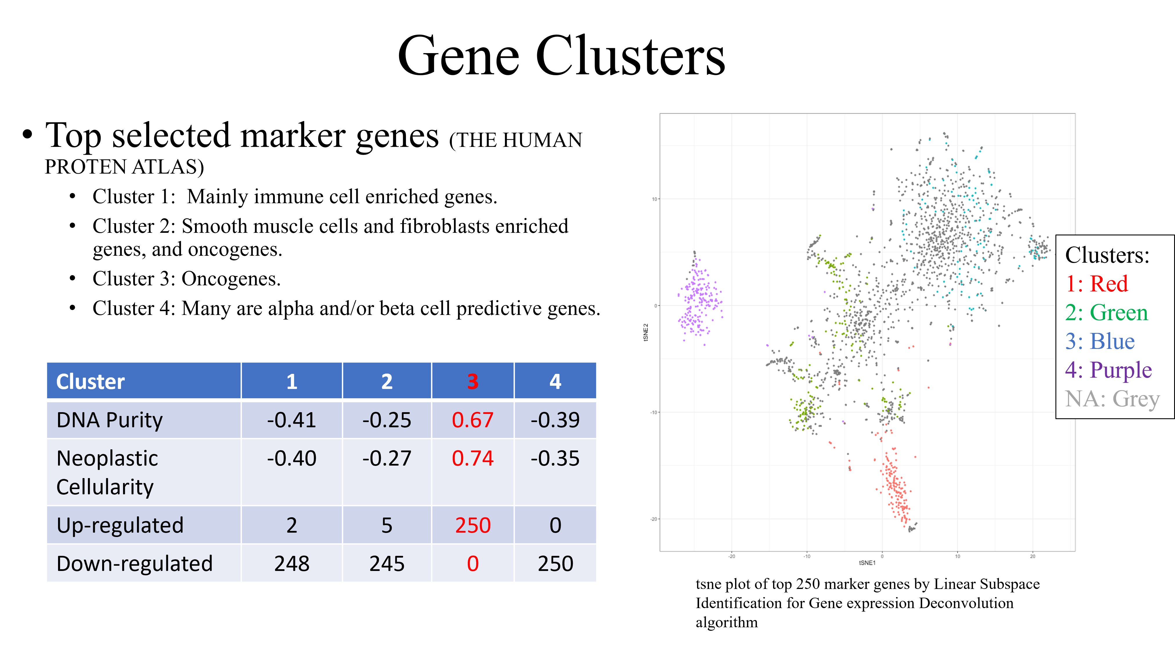
Gene clusters from analysis (II) provided insight into the genetic category that the consensus DE genes belong to. DNA purity values closer to 1 fit genes to a given cluster with more certainty. Neoplastic cellularity values indicate the average cancer purity value for the genes in that cluster. Here, the oncogene cluster stands out as the most prominent cluster for DE genes to reside in. This cluster contains the highest DNA purity and neoplastic cellularity levels with the greatest up-regulation.
Conclusion
This probability model study required the conduction of various simulation studies to test Poisson-Tweedie model performance. By applying the Poisson-Tweedie model to analyze a TCGA data set, I successfully detected 1403 promising differentially expressed genes associated with PDAC. I explored the functionals of both consensus and non-consensus DE genes. It is important to note that some of the non-consensus DE genes may be true marker genes of healthy cells. Further research could integrate this analysis with other genomic analyses for more insight into biological mechanisms underlying PDAC. The combination of neoplastic cellularity information and DE gene identification could possibly be considered under one unified mathematical model as well.