
Exploring the World of Markov Chains
Background
When building a discrete predictive model, it’s natural to assume that adding more features will improve performance. Complex neural networks in particular seem to demand large feature sets and deep historical data to generate accurate predictions. However, high performance doesn’t always require that degree of complexity.
A Stochastic Process describes a system where state changes are driven by probability. This type of process follows an assumption known as the Markov Property - the next state of the system depends only on the current state, not the sequence of prior states that led to the current state. This idea forms a core framework in probabilistic modeling.
A First-Order Markov Chain is a mathematical model that uses this property to predict the next state of a system given only its current state. Despite the simplicity in requiring no memory of past states, this approach can prove powerful across many applications, like natural language processing or predicting how users navigate websites.
The Basics of a Markov Chain
Before we look at a real-world application of a Markov chain model, let’s familiarize ourselves with some basic concepts. For any stochastic process, we must define the State Space S: a complete set of states covering all possible system outcomes. For example, let’s define a system with exactly three states. Then the state space S = {S1, S2, S3}. From any state Sn in S, the system can transition to one of the other two states, or remain in the same state.
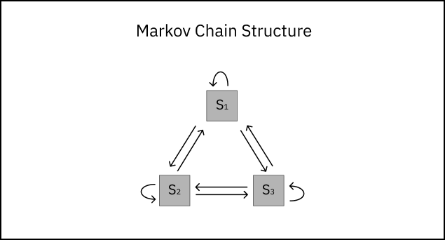
A transition from state i to state j is written as i→j. Consider a random state in our system like S1. From S1, there exist three possible transitions:
S1→S1 : starting from state S1, we stay in state S1.
S1→S2 : starting from state S1, we transition to state S2.
S1→S3 : starting from state S1, we transition to state S3.
![]()
Each transition i→j has a transition probability - the likelihood of transitioning from state i to state j. The transition probability Pij can be written as:
\[\normalsize P_{ij} \;=\; P(S_i \rightarrow S_j) \;=\; P\!\left(S_{t+1} = S_j \mid S_t = S_i\right), \qquad t \text{ = state step}\]In order to estimate the probability of a transition occuring, P̂ij, we must first observe the system and count the number of transitions from i→j that occur. These observable counts are denoted cij.
![]()
We’ll also need to count the number of transitions from i→k that have occurred, where k denotes any possible transition state from i. We can denote the total count of transitions from i as cik. Now, we’re ready to estimate the transition probability P̂ij. The maximum likelihood estimator for Markov chain transition probabilities is:
\[\normalsize \hat{P}_{ij} = \frac{c_{ij}}{\sum_{k} c_{ik}}\]Once calculating P̂ij for every possible transition in the system, we can update our original diagram with transition probabilities.
![]()
Note: The transition probabilities from any state add up to one, ensuring all possible next states are accounted for.
Application
Markov chain models are useful when a system’s future state depends primarily on its current state rather than its full history. Compared to more complex models, they require fewer features (and fewer assumptions about their correlations) while maintaining interpretability of state-to-state dynamics.
Let’s dive into a real use case: modeling user navigation on an online retailer website. As web users explore a retail site, they navigate through links on their way to completing a purchase. These interactions might be captured via clickstream logs or server-side analytics services. I simulated a dataset capturing 100,000 individual user sessions on a fictitious retail website: Ethan’s Marketplace (kudos for originality). Here’s a visual of our website’s homepage highlighting all possible user navigations (states) in this dataset.
UI design generated by Claude Sonnet 4.6
By defintion, every user journey will start on one of three pages: the homepage (95% of sessions), the search page (3%), or the customer support page (2%). Our simulated dataset contains only three columns.
session_id is the unique ID for each user session.
t is the click number from the start of a user session.
state is the web page the user navigates to.
Here’s an example of a single user session from the dataset.
| session_id | t | state |
|---|---|---|
| 6 | 0 | home |
| 6 | 1 | search |
| 6 | 2 | category |
| 6 | 3 | product |
| 6 | 4 | cart |
| 6 | 5 | checkout |
Now, let’s develop a Markov chain model to answer some questions regarding user behavior on our website.
Modeling
The first step in building our Markov chain will be identifying all transient and absorbing states from our state set S.
Transient States are states that the process can leave and possibly return to later.
Absorbing States are states that cannot be left. Once entered, it is impossible for the process to transition to another state.
In our model, reaching the checkout page will mark the end of a user session. Similarly, if a user leaves the site for any reason, their session will terminate immediately. Thus, we define two absorbing states in S: Checkout and Bounce. All remaining states will be defined as transient, since the user can navigate back to these states at any time. We’ll use this information to modifying the dataset slightly, creating state navigation paths (i→j) from each row. This will help us with counting individual transitions between states.
# Loading in our data...
df = pd.read_csv("userSessionLog.csv")

# Order dataset by session_id, then click event (this will help us define the 'next state' within row context)
df = df.sort_values(["session_id", "t"])

# Define states (pages) on the website
states = df['state'].unique().tolist()

# Create 'next state' value in the row
df["next_state"] = df.groupby("session_id")["state"].shift(-1)

# Drop rows that are final events (next state is null)
df = df.dropna(subset=['next_state'])

# Display cleaned dataset
df.display()
| session_id | t | state | next_state |
|---|---|---|---|
| 0 | 0 | home | search |
| 0 | 1 | search | category |
| 0 | 2 | category | category |
| 0 | 3 | category | category |
| 0 | 4 | category | bounce |
| 1 | 0 | home | search |
Next, we’ll define a Transition Probability Matrix for the Markov chain using counts of state transitions in our dataset. Think of this as an organized way of counting the observed transitions between states.
# Define the number of states in the model (8 in total)
n = len(states)

# Create an 8x8 array to count unique i->j state transitions from the dataset
counts = np.zeros((n, n), dtype=float)

# Map each state to an integer
S2I = {}
for i, s in enumerate(states):
    S2I[s] = i

# Using two arrays: from-states & to-states...
for s_from, s_to in zip(df["state"].to_numpy(), df["next_state"].to_numpy()):

    # ...Update counts of transitions from i to j in the counts matrix
    counts[S2I[s_from], S2I[s_to]] += 1.0

# Create counts as a dataframe
counts_df = pd.DataFrame(counts, index=states, columns=states)

# View the individual counts by i->j state transition
counts_df.display()
| home | search | category | bounce | product | cart | support | checkout | |
|---|---|---|---|---|---|---|---|---|
| home | 6,186 | 27,404 | 22,507 | 31,100 | 22,332 | 8,762 | 6,123 | 0 |
| search | 3,298 | 3,364 | 13,093 | 11,804 | 13,108 | 0 | 3,335 | 0 |
| category | 3,459 | 3,440 | 3,972 | 11,068 | 20,921 | 5,033 | 2,042 | 0 |
| bounce | 0 | 0 | 0 | 0 | 0 | 0 | 0 | 0 |
| product | 8,480 | 7,131 | 8,560 | 17,689 | 7,167 | 17,828 | 4,314 | 0 |
| cart | 988 | 0 | 0 | 5,701 | 5,933 | 2,729 | 2,503 | 16,498 |
| support | 6,891 | 3,739 | 1,803 | 6,140 | 1,708 | 0 | 1,466 | 0 |
| checkout | 0 | 0 | 0 | 0 | 0 | 0 | 0 | 0 |
From each state i (row) to state j (column), we observe these transition counts from the dataset. Observe that no transitions originate from either absorbing state — this is to be expected. Next, we’ll estimate transition probabilities using these counts for each state-to-state transition. Recall the formula for estimating the transition probability P̂ij:
\[\normalsize \hat{P}_{ij} = \frac{c_{ij}}{\sum_{k} c_{ik}}\]Keep in mind our probability estimates are only as reliable as the data behind them. Sure, we know definitively that transitions from absorbing states will always be zero. But what about the several instances above where we observe 0 transitions between transient states? No transitions exist from several states above, like cart → category. That doesn’t necessarily mean the move is impossible, just very unlikely. To avoid hard-coding impossibility, we can introduce a concept known as Laplace smoothing. This adds a small constant to every transition count from transient states, ensuring no probability is zero and all rows sum to one. This stabilizes estimates when some transitions are missing in the data.
\[\normalsize \hat{P}_{ij} = \frac{c_{ij} + \alpha}{\sum_{k} (c_{ik} + \alpha)}, \quad \text{where } i \text{ is a transient state}\]We’ll select an alpha value of 0.1 for smoothing. Now, time to build our transition probability matrix.
# Define a small alpha for Laplace smoothing
alpha = 0.1

# Define absorbing & transient states
absorbing_states = ["checkout", "bounce"]
transient_states = [i for i in states if i not in absorbing_states]

# Smooth counts for transitions from transient states
for s in transient_states:
    counts_df.loc[s, :] = counts_df.loc[s, :] + alpha

# Sum total counts by row
row_totals = counts_df.sum(axis=1)

# Renormalize rows in the transition probability matrix to get final estimate
P_hat_df = counts_df.div(row_totals.replace(0, np.nan), axis=0)

# Correct absorbing state probabilities
for s in absorbing_states:
    P_hat_df.loc[s, :] = 0
    P_hat_df.loc[s, s] = 1.0

# View transition probability matrix
display(P_hat_df)
| home | search | category | bounce | product | support | cart | checkout | |
|---|---|---|---|---|---|---|---|---|
| home | 5% | 22% | 18% | 25% | 18% | 5% | 7% | ≈0% |
| search | 7% | 7% | 27% | 25% | 27% | 7% | ≈0% | ≈0% |
| category | 7% | 7% | 8% | 22% | 42% | 4% | 10% | ≈0% |
| bounce | 0% | 0% | 0% | 100% | 0% | 0% | 0% | 0% |
| product | 12% | 10% | 12% | 25% | 10% | 6% | 25% | ≈0% |
| support | 32% | 17% | 8% | 28% | 8% | 7% | ≈0% | ≈0% |
| cart | 3% | ≈0% | ≈0% | 17% | 17% | 7% | 8% | 48% |
| checkout | 0% | 0% | 0% | 0% | 0% | 0% | 0% | 100% |
Great! Now that our Markov chain is complete, we can begin answering some questions around user behavior on the website. For example, if a user starts their session on the homepage, what is the probability they eventually checkout? We’ll answer this first question using some linear algebra and our knowledge of absorbing states.
Let \(P\) be the transition probability matrix of the Markov chain, partitioned into transient and absorbing states. Suppose there are t transient states and r absorbing states. Then \(P\) can be written in block form:
\[P = \begin{bmatrix} Q & R \\ 0 & I_r \end{bmatrix}\]Where:
- \(Q \in \mathbb{R}^{t \times t}\) contains transition probabilities between transient states.
- \(R \in \mathbb{R}^{t \times r}\) contains transition probabilities from transient to absorbing states.
- \(I_r\) is the \(r \times r\) identity matrix for the absorbing states.
- \(0\) is a zero matrix of size \(r \times t\).
The Fundamental Matrix \(N\) captures the expected number of visits to each transient state before absorption:
\[N = (I_t - Q)^{-1}\]Where \(I_t\) is the identity matrix of size \(t \times t\).
Finally, the absorption probabilities are computed as:
\[B = N \, R\]- Each entry \(B_{ij}\) is the probability that, starting from transient state \(i\), the chain is eventually absorbed in absorbing state \(j\).
- In our case, the probability that a session starting at home reaches checkout is:
Ah, beautiful math. With a few simple matrix operations, these formulas allow us to compute the probability of reaching checkout from the homepage.
# Rename P_hat_df for legebility
P = P_hat_df

# Define our starting & ending states
start_state = "home"

# Define Q: a 6x6 matrix of transition probabilities among the transient states
Q = P.loc[transient_states, transient_states].values

# Define R: a 6x2 matrix of transition probabilities from transient states to absorbing states
R = P.loc[transient_states, absorbing_states].values

# Define I: a 6x6 identity matrix
I = np.eye(Q.shape[0])

# Calculate the Fundamental matrix
N = np.linalg.inv(I - Q)

# Define B: a matrix of absorption probabilities from each transient state
B = N @ R

B_df = pd.DataFrame(
    B,
    index=transient_states,
    columns=absorbing_states
)

# Probability of eventually reaching checkout from homepage
prob_reach_checkout = B_df.loc[start_state, "checkout"]

# Survey says...
print(prob_reach_checkout)
The probability of eventually reaching checkout from the homepage is approximately 16.6%. Let’s validate from our observed counts in the dataset.
# Unique session IDs starting at home
home_session_ids = df.loc[(df["t"] == 0) & (df["state"] == "home"), "session_id"].unique()

# Count sessions that eventually reach checkout
checkout_session_ids = df.loc[df["next_state"] == "checkout", "session_id"].nunique()

# Probability of reaching checkout from home
prob = (checkout_session_ids / len(home_session_ids)) * 100

# Print the observed probability
print(prob)
The observed probability is 17.3% — that’s pretty close to our model’s estimate!
For any session starting from the homepage, what’s the expected number of clicks from the user before the session ends? Recall that every user session must end via a bounce or by reaching checkout. Easily enough, we can leverage the Fundamental matrix N to answer this question directly.
# Expected number of clicks to absorption from each transient state
expected_clicks = N.sum(axis=1)

# Convert to a DataFrame for legibility
expected_clicks_df = pd.DataFrame(expected_clicks, index=transient_states, columns=["clicks"])

# Expected clicks starting from home
expected_clicks_home = expected_clicks_df.loc[start_state, "clicks"]

# Output the expected clicks to absorption starting from home
print(expected_clicks_home)
Starting from the home page, the expected number of clicks to reach checkout or bounce is 3.49. This estimate is close to the observed average clicks from the dataset, 3.66.
Let’s consider one last scenario. Say we run an advertisement on the category page to promote products. How many checkout conversions can we expect to come from users who went through the category page? This might give us a sense of the advertisement’s impact on buyers. We’ll answer this question using conditional probability. What’s the chance a user visited the category page given they reached checkout.
\[p(a \mid b) = \frac{p(a \text{ and } b)}{p(b)}\] \[p(\text{category} \mid \text{checkout}) = \frac{p(\text{category and eventually checkout})}{p(\text{eventual checkout})}\] \[p(\text{category} \mid \text{checkout}) \approx \frac{N[\text{home}, \text{category}] \cdot B[\text{category}, \text{checkout}]}{B[\text{home}, \text{checkout}]}\]# Define fundamental matrix clicks dataframe
n_df = pd.DataFrame(N, index=transient_states, columns=transient_states)
# Define absorption probability dataframe
b_df = pd.DataFrame(B, index=transient_states, columns=absorbing_states)
# Estimate the probability of visiting the category page given eventual checkout
p_category_given_checkout = (
n_df.loc["home", "category"] * B_df.loc["category", "checkout"] / B_df.loc["home", "checkout"]
)
# View model estimate
print(f"Markov chain estimate: {p_category_given_checkout:.2%}")
Markov Chain Estimate: 59.83%
About 60% of sessions that end in checkout pass through the category page along the way. That means most buyers are exposed to products at the category level before converting. This insight might help us determine how to price and position new advertisements shown on this page in the future.
A Markov chain model can be a powerful tool that eliminates the cost of complexity and resources. Sometimes, the simplest model might just be the smartest one.