Rethinking A/B Testing with Bayesian Inference

Background

Running an A/B test sounds straightforward. Split your test data, measure an outcome, and pick a winner. Yet assumptions in the most common A/B tests can break down in ways that are easy to miss and costly to ignore. Luckily, there are alternative approaches that treat belief as something to be updated as evidence arrives, rather than a mere threshold to be crossed. In this post, we’ll build our knowledge on the Bayesian statistical framework and examine what it really costs to get decisions wrong.

The Issue with Frequentist Probability

The Frequentist definition of probability is the most widely known in statistics. It states that probability measures the long-run frequency of an event occurring over many repeated trials. A classic example is the coin flip. Flipping a coin millions of times, the proportion of heads gradually stabilizes near 0.5 as an estimate of the true underlying probability. That true probability is always unknown, but with enough repeated trials, we can get reasonably close.

Frequentist A/B Testing is an experiment we run to see if two processes behave significantly differently from one another. Consider a pharmaceutical company testing a new treatment to relieve headaches. Patients are randomly assigned to receive treatment A (an existing medication) or treatment B (the new medication). After exposure to the treatment, each patient reports whether their headache was relieved within one hour. The goal of this test is to determine whether treatment B produces a meaningfully higher relief rate than treatment A. The null hypothesis for this A/B test is: Treatments A and B produce identical relief rates. We’d then define a fixed number of patients, each receiving exactly one of the two treatments. Then, we’d use the test results to compute a single p-value answering the question: What’s the probability of observing data as extreme as ours if the null hypothesis is true? If this probability is very unlikely (< 0.05), we’d reject the null hypothesis and claim that the two treatments produce meaningfully different relief rates, resulting in a winner.

Key takeaways on the Frequentist A/B approach:

• The p-value from this test is the probability of observing our collected data given the null hypothesis is true.
• Frequentist probability treats the true relief rates of treatments A and B as fixed, unknown constants (probabilities that do not change).
• The false positive rate (0.05) is only controlled in the test if we commit to our sample size in advance and look at the results exactly once.

Let’s say we decide a reasonable sample size for this experiment to be 500 patients. As we carry out this experiment, stakeholders behind the scenes are eager to monitor the results in real time. After the first 50 sessions, the resulting p-value dips to 0.03, indicating we should reject the null hypothesis and favor treatment B. The issue is, every time we glance at the accumulating results before reaching our defined sample size of 500, we risk rejecting the null hypothesis by chance alone. This is known as p-hacking by peeking, which can actually inflate the 0.05 false positive rate we thought we were controlling. Research suggests that peeking at live results just ten times can balloon a 0.05 false positive rate to upwards of 0.25 (Miller, 2010). So why peek at all? Interim results can be tempting to those who have incentive to act on promising data early, even when the data isn’t fully conclusive. Frequentist A/B testing is meant for a world where we resist that pressure, but that’s not always the case in practice.

After 100 sessions, treatment B has a relief rate of 68% and treatment A has a relief rate of 61%. Is treatment B truly better yet? If we’re playing by the frequentist rules, we’re in a tough spot. We’ve been monitoring the number of collected sessions, but we still haven’t reached our pre-defined sample size of 500 (and frankly, we’re questioning whether 100 independent patient sessions could have been a sufficient sample size to begin with). At this point, the p-value still cannot tell us: Given the data, how confident should we be that treatment B is genuinely better? Lucky for us, Bayesian inference can help us answer this question.

What is Bayesian Statistics?

The Bayesian definition of probability is a measurement of belief. It represents a value of uncertainty about an event, whether it happens once or many times. Our belief in the outcome of an event can change as we observe new evidence. Instead of committing to a single fixed estimate, we maintain a full distribution of beliefs across all possible parameter values, updating these beliefs as new evidence arrives.

Let’s revisit the coin flip for a moment. Under frequentist thinking, we flip a coin millions of times, and the probability of landing on heads will converge to a fixed value around 0.5. With Bayesian probability, we start with a belief about the coin’s bias, like “I expect the true probability of landing on heads to fall between 0.4 and 0.6.” We might suspect the coin is fair, but we’re not certain. Well, we can revise that belief with every flip. After 10 flips, our distribution is wide and uncertain. After 10,000 flips, it has narrowed considerably. While both Frequentist and Bayesian estimates in this example might lead to the same result, the Bayesian approach allows us to carry a full picture of our estimates and uncertainty along the way.

We’ll use this same approach now for the clinical drug experiment. Instead of asking whether the relief rate of treatment B is significantly different than treatment A at some fixed sample size, we’ll construct a distribution of beliefs around both treatments’ true relief rates, updating both in real time as patient sessions are recorded. To understand how that updating works, we need Bayes’ Theorem. Let’s recall our favorite conditional probability formula:

\[\small P(A \mid B) = \frac{P(B \mid A) \cdot P(A)}{P(B)}\]

In our experiment, we’re not talking about abstract events A and B. We care about parameters and data. Let’s rewrite this formula as:

\[\small P(\theta \mid X) = \frac{P(X \mid \theta) \cdot P(\theta)}{P(X)}\]

Where θ is the unknown parameter we want to learn (the true relief rate for a particular treatment) and X is the observed data (the recorded outcomes of relieved and not relieved from real patient sessions).

Next, we need to define a few new terms:

Term	Name	Definition
\(P(\theta)\)	Prior	Our belief about θ before seeing any data
\(P(X \mid \theta)\)	Likelihood	How probable is this data, given a particular value of θ?
\(P(\theta \mid X)\)	Posterior	Our updated belief about θ after seeing the data
\(P(X)\)	Marginal Likelihood	A normalizing constant that ensures the posterior is a valid distribution

The posterior is always what we’re after. It reflects our updated belief about θ given everything observed so far.

Let’s put this knowledge to the test with a famous example in Bayesian probability.

---

Consider a disease that affects 1% of the population. A diagnostic test for this disease is 95% accurate: if you have the disease, the test returns positive 95% of the time. If you don’t have the disease, the test returns negative 95% of the time (a 5% false positive rate). You test positive. What is the probability you actually have the disease?

Here’s how we go about answering this question using the formulas above.

\[\small \begin{aligned} P(\theta) &= 0.01 \quad \text{(prior: 1% of the population has the disease)} \\ P(X \mid \theta) &= 0.95 \quad \text{(likelihood: test returns positive 95% of the time given disease is present)} \end{aligned}\]

Expanding $P(X)$ using the law of total probability:

\[\small \begin{aligned} P(X) &= P(X \mid \theta)P(\theta) + P(X \mid \neg\theta)P(\neg\theta) \\ &= (0.95)(0.01) + (0.05)(0.99) = 0.0095 + 0.0495 = 0.059 \end{aligned}\]

Drumroll…

\[\small P(\theta \mid X) = \frac{0.95 \times 0.01}{0.059} \approx 0.161\]

There’s actually only a 16% chance you have the disease despite a 95% accurate test. Many people (my initial self included) assume the answer is closer to 95%. The disease is so rare that false positives outnumber true positives across the full population. Our prior belief (only 1% of people have this disease) is powerful enough to override a test that is 95% accurate. Thus, the posterior is a balance between prior belief and observed evidence. If you were to test positive twice in a row, that posterior of 16% becomes your new prior going into the next update. Each result reshapes your belief, which becomes the starting point for the next posterior.

---

A side note on the marginal likelihood P(X)

Notice P(X) sits in the denominator of the posterior formula above. Its only job is to ensure the posterior sums to 1 across all possible values of θ. It has no dependence on θ and is a constant regardless of the parameter value we're evaluating. Since we'll be focused on identifying the shape of the posterior distribution, a constant that scales everything uniformly doesn't meaningfully change anything. We can drop the denominator and write: $$ \small P(\theta \mid X) \propto P(X \mid \theta) \cdot P(\theta) $$

Where ∝ means "proportional to"

Again, the shape of the posterior is determined entirely by the numerator, so we'll refer to this formula from here on out.

Recall Frequentist probability views the true relief rate of treatment B as a fixed, unknown constant. We can only estimate this true relief rate by collecting data, running a test, and arriving at a single value like 68%. We can add a confidence interval around our estimate, but we’re ultimately left with a single estimate and a range. There’s no formal way for us to say we believe the true rate is probably around 68% with a reasonable chance it’s as high as 75%. We can’t update that estimate fluidly as new sessions arrive either. The Bayesian play is to represent θ (the true relief rate) as a probability distribution. Instead of committing to a single estimate, we capture a full distribution of our uncertainty across every possible value between 0 and 1. The mean of the distribution is where we think the true θ value most likely falls. The width of the distribution reflects how certain or uncertain we are. Whenever new data arrives and we update our prior, the entire distribution updates.

A Beta Distribution $\text{Beta}(\alpha, \beta)$ is a common probability distribution in Bayesian statistics defined on the interval [0,1]. The distribution uses two parameters, α (alpha) and β (beta), to represent pseudo-counts of successes and failures measuring θ. We can use this distribution to model our prior belief of θ. For example, think of α as the number of relieved outcomes (successes) and β as the number of non-relieved outcomes (failures) before the clinical drug experiment begins. A $\text{Beta}(1, 1)$ prior represents starting as if we’ve seen exactly one success and one failure (essentially no prior bias). A $\text{Beta}(10, 30)$ represents having already observed 10 successes from 40 sessions, suggesting a prior belief of roughly 25% relief rate with moderate confidence.

If we have no prior beliefs on the true relief rates of treatments A or B at the start of the A/B test, we can use the neutral $\text{Beta}(1, 1)$ as the prior for both treatments. This is a flat, uninformative prior telling the model we have no strong belief about the effectiveness of either treatment before the experiment. After 500 sessions are collected for each treatment, each success and failure to relieve a headache would update the corresponding Beta posterior distributions (one for $\theta_A$, one for $\theta_B$). We’d then ask what the probability is that a sample drawn from B’s posterior exceeds a sample drawn from A’s posterior.

The probability density function for the Beta distribution is:

\[\small f(\theta \mid \alpha, \beta) = \frac{\theta^{\alpha-1}(1-\theta)^{\beta-1}}{B(\alpha, \beta)}\]

Where $B(\alpha, \beta)$ is the normalizing constant ensuring the distribution integrates to 1 over [0,1]. This is analogous to P(X) in Bayes’ theorem. When we plot the Beta distribution, θ sits on the x-axis. We’re never claiming we know θ. Instead, we’re asking how likely each possible value of θ is given our current beliefs. We’ll take a look at a few of these plots below. Try thinking of them as pictures of uncertainty around the true value of θ.

Here are some examples of a prior $\text{Beta}(\alpha, \beta)$ distribution for the relief rate of treatment B. The peak location is always $\alpha/(\alpha+\beta)$. The width tells us how much volatility is behind that belief.

Beta(1, 1) — An uninformative prior

This is a completely flat distribution. Every possible relief rate from 0 to 1 is equally likely. We’re essentially expressing no prior belief about what to expect.

Beta(13, 7) — A weak prior belief

Equivalent to observing 13 relieved outcomes from 20 sessions. Soft belief that treatment B’s relief rate is around 65%.

Beta(204, 96) — A strong prior belief

Equivalent to 204 relieved outcomes from 300 sessions. High confidence that treatment B’s relief rate is near 68%.

Now, here’s where the math gets exciting. If we pair the right prior $P(\theta)$ with the right likelihood $P(X \mid \theta)$, the posterior comes out as the same family of distributions as the prior. This is called Conjugacy, and it’s what makes our update rule clean enough to derive by hand. In the clinical drug experiment, our likelihood comes from a binomial distribution (relieved or not relieved being the binary outcome) and the prior comes from a $\text{Beta}(\alpha, \beta)$ distribution (defined on the closed $[0,1]$ interval for probability). Together, they form a Beta-Binomial conjugate pair, which can be used to update the prior.

Let’s break down how this works. Consider the likelihood $P(X \mid \theta)$. If we observe n patient sessions for a particular treatment with k successful relief outcomes, the likelihood of this data given a particular value of θ is:

\[\small P(X \mid \theta) = \binom{n}{k} \theta^k (1-\theta)^{n-k}\]

This is the Binomial distribution. It answers the question of how probable it is to observe exactly $k$ relief outcomes from $n$ sessions, given a true relief rate of $\theta$. Notice that $\binom{n}{k}$, the binomial coefficient, is only a constant with no dependence on $\theta$. Just like $P(X)$ in Bayes’ theorem, we can drop it when reasoning about the shape of the posterior. So, the likelihood simplifies to:

\[\small P(X \mid \theta) \propto \theta^k (1-\theta)^{n-k}\]

To determine the Posterior $P(\theta \mid X)$, we must multiply the likelihood above with our Beta prior. Recall this prior takes the form:

\[\small P(\theta) \propto \theta^{\alpha-1}(1-\theta)^{\beta-1}\]

Multiplying likelihood by prior:

\[\small P(\theta \mid X) \propto \theta^k(1-\theta)^{n-k} \cdot \theta^{\alpha-1}(1-\theta)^{\beta-1}\]

Collecting exponents:

\[\small P(\theta \mid X) \propto \theta^{\alpha+k-1}(1-\theta)^{\beta+n-k-1}\]

Upon simplifying, this looks exactly like our Beta distribution, just with updated parameters:

\[\small P(\theta \mid X) = \text{Beta}(\alpha + k, \ \beta + n - k)\]

That’s the entire update rule! For a specific treatment in the experiment, our prior was $\text{Beta}(\alpha, \beta)$. We observe $k$ relieved outcomes from $n$ sessions for that treatment. So, our final posterior is $\text{Beta}(\alpha + k, \ \beta + n - k)$.

Here’s an example of how our belief in the true relief rate of treatment B can change as we accumulate data and update our prior with the latest posterior.

Sessions	Relieved Patients	Non-Relieved Patients	Posterior	Distribution Mean
0	0	0	$\text{Beta}(1, 1)$	0.500
10	7	3	$\text{Beta}(8, 4)$	0.667
50	34	16	$\text{Beta}(35, 17)$	0.673
100	68	32	$\text{Beta}(69, 33)$	0.676
500	340	160	$\text{Beta}(341, 161)$	0.680

Notice the mean of the posterior converges to the true relief rate as we accumulate more patient sessions. Each row’s posterior becomes the prior for the next update. The first prior’s influence pulling the mean towards 0.5 fades quickly as real data accumulates — by session 500, the data has taken over entirely. In the clinical drug experiment, we run this update simultaneously for both treatments, maintaining $\text{Beta}(\alpha_A, \beta_A)$ and $\text{Beta}(\alpha_B, \beta_B)$ in parallel. Every session that arrives updates one of the two distributions depending on which treatment was prescribed. We are never forced to wait for a pre-defined sample size, and the posteriors simply reflect whatever evidence we’ve seen so far.

Making Decisions Under Uncertainty

At any point in the clinical drug trial, we’ll have two posterior distributions.

\[\text{Beta}(\alpha_A, \beta_A) \text{ for treatment A.}\] \[\text{Beta}(\alpha_B, \beta_B) \text{ for treatment B.}\]

Either distribution represents our full belief about that treatment’s true relief rate at that point in the experiment. However, these distributions aren’t enough to guide decisions yet. When a stakeholder asks if treatment B is truly better than treatment A, we must answer two questions first.

• Given the latest data, how likely is it that treatment B is truly better than A?
• What would a wrong decision in the experiment cost us?
• To answer question 1…
  
  A Frequentist 95% confidence interval built around an estimated relief rate won’t tell us there’s a 95% probability the true rate lives inside it. It means that across many repeated experiments, 95% of the constructed intervals would contain the true rate. The true relief rate is always fixed in this lens. A specific confidence interval has it or it doesn’t, and frequentist statistics doesn’t allow us to assign a probability to that.

A Bayesian 95% credible interval is exactly what it sounds like. Given the data observed, there is a 95% probability that the true relief rate lies within this range. In the clinical drug trial, by the time treatment B’s posterior is $\text{Beta}(341, 161)$, we can hand a stakeholder a credible interval and say with confidence exactly where the true relief rate most likely falls.

With two independent Beta posterior distributions, we want to know how often a sample drawn from B’s posterior would exceed a sample drawn from A’s posterior. This can be denoted:

\[\small P(\theta_B > \theta_A)\]

Analytically, this is computed by integrating over all possible values of $\theta_A$ and $\theta_B$:

\[\small P(\theta_B > \theta_A) = \int_0^1 \int_{\theta_A}^1 f(\theta_B) f(\theta_A) \, d\theta_B \, d\theta_A\]

The double integral may look intimidating, but the intuition is straightforward. If treatment B’s posterior is almost entirely to the right of treatment A’s on the relief rate axis, P(B>A) approaches 1. If the two distributions heavily overlap, P(B>A) hovers near 0.5, meaning the data hasn’t separated them yet. P(B>A) is useful, but it is not quite the right number to make a final decision on.

To answer question 2…

P(B>A) = 0.95 might sound compelling, but what if treatment B is only 0.1% better than treatment A in the scenarios where it wins and 5% worse in the scenarios where it loses? Calling treatment B better might still be the wrong call. This is where expected loss comes in. What is the average cost of making the wrong decision?

We can define a loss function for each possible decision (choosing treatment A or B as superior). In either case, the loss measures how much effectiveness we leave on the table by promoting the inferior treatment. If we promote treatment B and it turns out to be worse, the loss is how much A exceeded B. If we promote treatment A and it turns out to be better, the loss is how much B exceeded A.

If we were to promote treatment B:

\[\small \mathcal{L}(\text{promote B}) = E[\max(\theta_A - \theta_B, 0)]\]

Similarly, if we were to promote treatment A:

\[\small \mathcal{L}(\text{promote A}) = E[\max(\theta_B - \theta_A, 0)]\]

We would only decide to promote Treatment B if the expected loss falls below some acceptable threshold ε:

\[\small \mathcal{L}(\text{promote B}) < \varepsilon\]

For simplicity, we use a shared threshold ε since treatment A is already the incumbent treatment. We could technically introduce a separate ε for promoting an alternative depending on the experiment.

Remember that Frequentist A/B testing should never allow early stopping in an experiment. The moment we break our commitment to the sample size, our false positive rate inflates and the results become unreliable. Under a Bayesian A/B test, we can stop as soon as the expected loss drops below ε. Whether it takes 100 or 1,000 sessions in the clinical drug experiment, the data will tell us once we’ve collected enough of it.

Tying It All Together

Let’s close with one last scenario. Imagine you’re a data scientist working for a video streaming platform. The platform recommends new content to viewers as soon as they finish watching a video. You’ve built a new recommendation model and want to know if it drives more clicks than the existing one.

Model A is the existing model. It recommends content based on what similar viewers have watched. Model B is your new model. It factors in how long the viewer watched their last video and whether they’ve rewatched content before. Both models show a ranked list of recommendations at the end of every video. The metric is simple enough. Did the viewer click on at least one recommended video?

We can carry out a simulation exposing 500 viewer sessions to each model. The key unknown in this experiment is the click-through rate (CTR) generated by each model’s recommendation. For our purposes, we’ll set the ground truth CTR for Models A and B at 25% and 28% respectively. This is a modest lift, but reasonable in practice. A 3% difference is meaningful at scale, but subtle enough to go undetected in the early stages of an experiment. That’s what will make this an interesting test case.

Let’s fire up our Python IDE to get started. We’ll first need to simulate viewer session outcomes from the ground truth Binomial distributions of each model.

# Import libraries
import numpy as np
from scipy import stats
import matplotlib.pyplot as plt
from scipy.special import betaln
from scipy.stats import chi2_contingency
 
# Set seed
np.random.seed(100)
 
# Pre-defined click through rates for simulation (unknown during experiments)
true_ctr_a = 0.25
true_ctr_b = 0.28
 
# Number of viewer sessions exposed to each model
n_sessions = 500
 
# Simulate binary outcomes for each model
clicks_a = np.random.binomial(1, true_ctr_a, n_sessions)
clicks_b = np.random.binomial(1, true_ctr_b, n_sessions)
 
# Print results
print(f"Model A: {clicks_a.sum()} clicks from {n_sessions} sessions "
      f"(observed CTR: {clicks_a.mean():.3f})")
 
print(f"Model B: {clicks_b.sum()} clicks from {n_sessions} sessions "
      f"(observed CTR: {clicks_b.mean():.3f})")

Model A: 124 clicks from 500 sessions (observed CTR: 0.248)
Model B: 132 clicks from 500 sessions (observed CTR: 0.264)

We’ll now define a few functions to call later in the script. These pull from everything we’ve covered about Bayesian inference so far.

# Create a function to update priors from observed data
def update_posterior(alpha, beta, click):
    """
    Update a Beta posterior given a single binary outcome.
    click = 1 (clicked) increments alpha (successes)
    click = 0 (no click) increments beta (failures)
    """
    alpha += click
    beta += 1 - click
    return alpha, beta
 
# Create a function to calculate the mean of a posterior distribution
def posterior_mean(alpha, beta):
    return alpha / (alpha + beta)
 
# Create a function to calculate the variance of a posterior distribution
def posterior_variance(alpha, beta):
    return (alpha * beta) / ((alpha + beta) ** 2 * (alpha + beta + 1))
 
# Create a function to return a credible interval containing 95% of the posterior distribution's belief about theta
def credible_interval(alpha, beta, credibility=0.95):
    lower = (1 - credibility) / 2
    upper = 1 - lower
    return stats.beta.ppf([lower, upper], alpha, beta)
 
# Create a function to sample n theta values from a Beta posterior distribution
def sample_posterior(alpha, beta, n=100_000):
    return np.random.beta(alpha, beta, n)
 
# Create a function to compute P(theta_B > theta_A) for two Beta distributions
def prob_b_beats_a(alpha_a, beta_a, alpha_b, beta_b):
    total = 0.0
    """
    Sum over each possible success count in B's posterior
    Given i successes for B, how much of A's distribution falls below that probability?
    betaln computes log Beta function values to keep numbers stable at large alpha/betas
    """
    for i in range(alpha_b):
        total += np.exp(
            betaln(alpha_a + i, beta_a + beta_b) -
            np.log(beta_b + i) -
            betaln(1 + i, beta_b) -
            betaln(alpha_a, beta_a)
        )
    return total

Unlike the last $P(B > A)$ function above, the expected loss integral doesn’t have a clean closed-form solution. We’ll use Monte Carlo sampling to draw a large number of θ (CTR) values from both posteriors, comparing them element-wise to simulate the joint distribution of $(\theta_A, \theta_B)$ and estimate expected loss directly. The law of large numbers guarantees this estimate converges to the true expectation quickly. 100,000 samples will be plenty!

def expected_loss(alpha_a, beta_a, alpha_b, beta_b, n_samples=100_000):
    """
    Estimate expected loss for promoting B and promoting A
    via Monte Carlo sampling over the joint posterior.
    """
    samples_a = sample_posterior(alpha_a, beta_a, n_samples)
    samples_b = sample_posterior(alpha_b, beta_b, n_samples)
 
    # Cost of promoting B: how much does A exceed B when A is better?
    loss_promote_b = np.mean(np.maximum(samples_a - samples_b, 0))
 
    # Cost of promoting A: how much does B exceed A when B is better?
    loss_promote_a = np.mean(np.maximum(samples_b - samples_a, 0))
 
    return loss_promote_b, loss_promote_a

The result of this expected loss function is only useful when paired with a threshold. Recall from earlier that we define an acceptable threshold ε and only promote Model B if the expected loss of shipping Model B is less than ε. We’ll set ε equal to 0.5%, meaning we’re willing to accept a 0.5% hit to our clickthrough rate if we accidentally promote the wrong model.

# Maximum acceptable CTR loss
epsilon = 0.005

Assuming we have no prior beliefs about the effectiveness of Model B, we’ll initialize its prior distribution as $\text{Beta}(1, 1)$. For Model A, its prior performance in production will help construct our prior belief. Let’s represent this belief in Model A’s CTR with a $\text{Beta}(1, 3)$ distribution.

# Initialize Beta(1,3) prior for Model A (estimating a 25% CTR)
alpha_a, beta_a = 1, 3
 
# Initialize Beta(1,1) prior for Model B (flat, unbiased)
alpha_b, beta_b = 1, 1

Next, let’s create a dictionary that logs the evolution of each posterior distribution as data accumulates.

# Track experiment history session by session
history = {
    "sessions": [],
    "mean_a": [],
    "mean_b": [],
    "prob_b_beats_a": [],
    "loss_promote_b": [],
    "loss_promote_a": [],
    "decision_made": None
}
 
# Record initial priors before any data arrives
history["sessions"].append(0)
history["mean_a"].append(posterior_mean(alpha_a, beta_a))
history["mean_b"].append(posterior_mean(alpha_b, beta_b))
history["prob_b_beats_a"].append(prob_b_beats_a(alpha_a, beta_a, alpha_b, beta_b))
history["loss_promote_b"].append(0.0)
history["loss_promote_a"].append(0.0)

As you and I know at this point, Model B is the superior model, so we’ve shaped some of our functions and simulation results around capturing when we’ve confidently observed this outcome.

Let’s run our first simulation to see when Model B proves victorious in the A/B test!

for t in range(1, n_sessions + 1):
 
    # Update each posterior with the current session outcome
    alpha_a, beta_a = update_posterior(alpha_a, beta_a, clicks_a[t-1])
    alpha_b, beta_b = update_posterior(alpha_b, beta_b, clicks_b[t-1])
 
    # Compute P(B > A) and expected loss at this point in the experiment
    p_b_wins = prob_b_beats_a(alpha_a, beta_a, alpha_b, beta_b)
    loss_b, loss_a = expected_loss(alpha_a, beta_a, alpha_b, beta_b)
 
    # Record metrics for the current session
    history["sessions"].append(t)
    history["mean_a"].append(posterior_mean(alpha_a, beta_a))
    history["mean_b"].append(posterior_mean(alpha_b, beta_b))
    history["prob_b_beats_a"].append(p_b_wins)
    history["loss_promote_b"].append(loss_b)
    history["loss_promote_a"].append(loss_a)
 
    # Promote Model B when expected loss clears epsilon
    if history["decision_made"] is None and loss_b < epsilon:
        history["decision_made"] = t
        print(f"Decision at session {t}: Promote Model B")
        print(f"P(B > A):          {p_b_wins:.4f}")
        print(f"Expected loss:     {loss_b:.5f}")
        print(f"Posterior mean A:  {posterior_mean(alpha_a, beta_a):.4f}")
        print(f"Posterior mean B:  {posterior_mean(alpha_b, beta_b):.4f}")

Decision at session 169: Promote Model B
 
P(B > A): 0.8267
Expected loss: 0.00429
Posterior mean A: 0.2254
Posterior mean B: 0.2690

By session 169, the expected loss drops below ε, triggering an early decision in favor of Model B. As you can see above, the posterior means didn’t converge to their true CTR values yet. We’re only stating the scenarios sampled from both posteriors produced an acceptably low cost of being wrong about promoting Model B. The Bayesian framework didn’t wait for certainty around the CTR estimates. Instead, the test stopped when the risk of a wrong decision became tolerable.

To put the Bayesian approach in context, let’s run the same simulation as a Frequentist A/B test. We’ll use a Chi-square test to evaluate results at exactly 169 sessions, with a fixed sample size of 500 viewer sessions per model. Stopping here (peeking early) will highlight just how differently the two frameworks interpret the same underlying data.

# Run frequentist chi-square test on data up to the Bayesian decision point
t_decision = history["decision_made"]
 
# Build a contingency table to run the chi-square test on
contingency = np.array([
    [clicks_a[:t_decision].sum(), t_decision - clicks_a[:t_decision].sum()],
    [clicks_b[:t_decision].sum(), t_decision - clicks_b[:t_decision].sum()]
])
 
# Results
chi2, p_value, _, _ = chi2_contingency(contingency)
print(f"Frequentist test at session {t_decision} (Peeking Early):")
print(f"Chi-square statistic: {chi2:.4f}")
print(f"p-value:              {p_value:.4f}")
print(f"Significant at 0.05:  {p_value < 0.05}")

Frequentist test at session 169 (Peeking Early):
 
Chi-square statistic: 0.5749
p-value: 0.4483
Significant at 0.05: False

By session 169 in the Frequentist test, a p-value of 0.45 is nowhere near a 0.05 threshold. The test can’t reject the null hypothesis at this point. It demands more data before drawing any meaningful conclusion.

The Bayesian framework reached a decision at that same session without violating a single assumption. It’s worth noting again: $P(B > A)$ never crossed 0.95 across the entire experiment. The decision wasn’t driven by confidence in the direction of the result. It came down to the expected cost of promoting the wrong model falling below what we were willing to accept. Here’s how that played out across all 500 sessions.

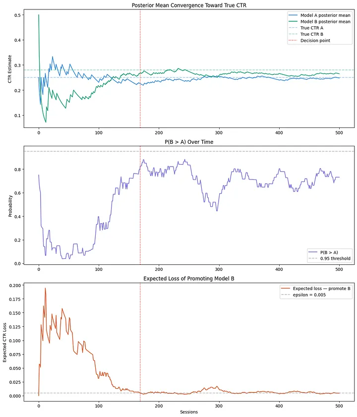
Plot 1 shows both posterior means converging toward the true CTR values over time. Increasing the number of viewer sessions from 500 to 1,000 would get us even closer to 0.25 and 0.28.

In plot 2, $P(B > A)$ spends a long stretch below 0.5 early on. The data briefly favored Model A before enough evidence accumulated to separate the two models. You’ll notice it never crosses 0.95, highlighting why expected loss is the better decision criterion.

Plot 3 tells the clearest story. Expected loss starts high and noisy, then steadily falls as the posteriors sharpen. It crosses epsilon at session 169 and lands us at our answer to promote Model B.

Bayesian statistics gives us a principled way to make decisions under uncertainty without the constraints of frequentist testing. We maintain a full distribution of beliefs about unknown parameters and update them continuously as new evidence arrives. This lets us answer questions that actually matter in practice. The expected loss framework takes it one step further, replacing an arbitrary significance threshold with a concrete measure of what being wrong actually costs. Next time you’re tempted to peek at that p-value, maybe just let the posterior do the talking.